Download
1 / 1
10 likes | 130 Vues
Monitoring atmospheric gravity waves by means of SAR, MODIS imagery and high-resolution ETA atmospheric model: a case study M. Adamo (1), G. De Carolis (1), S. Morelli (2), F. Parmiggiani (3)

E N D
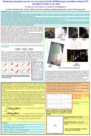
Monitoring atmospheric gravity waves by means of SAR, MODIS imagery and high-resolution ETA atmospheric model: a case study M. Adamo (1), G. De Carolis (1), S. Morelli (2), F. Parmiggiani (3) (1) ISSIA-CNR, Bari, Italy, (2) Dept. of Physics, University of Modena and Reggio Emilia, Italy, (3) ISAC-CNR, Bologna Italy 10:40 MODIS02 Composite Image 10:08 ERS-2 SAR Image Figure 1. Temporal sequence of satellite images. The periodic cloud pattern between Corsica peninsula and Elba Island (visible on NOAA/AVHRR and MODIS images at 1Km and 250 m of spatial resolution respectively) is the manifestation of the atmospheric gravity wave generated by orographic interaction of the western air flow with Corsica peninsula. The cloud pattern is about 180° out of phase with corresponding bright streaks revealed on SAR image. The wavelength is about 15 Km. The gravity wave phenomenon started earlier as documented by AVHRR image acquired at 03:17 UTC over the same area. In correspondence to the Ligurian Gulf on the ERS-2 SAR images, ETA wind vectors (green arrows) and CMOD–4 retrieved wind vectors (yellow arrows) are represented for comparison. AGW model description When air flow impinges upon a terrain obstacle, the disturbance causes displacement of the air from equilibrium position in the lee side of the obstacle. As a result, air parcels start to oscillate generating internal atmospheric waves restored by gravity. If lee waves propagate over the ocean surface, the corresponding wind speed variation modulates the local surface roughness, which is in turn detected as NRCS modulation on SAR images. Air flow downstream the terrain barrier is modeled on the following assumptions: 1) the barrier is infinitely long and approximated by a bell-shaped function; 2) the wind blows parallel to the short side of the barrier. In the reference bi-dimensional Cartesian space x-z, where x is the downstream direction and z is the vertical direction pointing upwards from the ground placed at z=0, the two-dimensional air parcel oscillations can be described by the Scorer parameter where is the atmospheric stability parameter; U=U(z), (z) are the horizontal wind speed and the potential temperature upstream the barrier; g is the acceleration due to gravity. The Scorer parameter in the lower atmosphere up to about 10 Km can be usually represented by the exponential function l(z)=l(0)exp(-cz), even if abrupt changes of l due to thin inversion layers may occur. As a result, the wave-like solution of the horizontal velocity u modulating the upstream wind speed U can be written as [4]: for a bell-shaped ridge B(x,0)=Hb2/(b2+x2) for a Gaussian-shaped ridge G(x,0)=Hexp(-a2x2) is the exponent of the adiabatic atmosphere (z)=(0)exp(- z). The sum is performed on the resonant wave-numbers forming the lee wave pattern obtained as solution of the equation: where J denotes the Bessel function of the first kind. (1) ABSTRACT Results of an experiment for surface wind field retrieval in presence of an atmospheric gravity wave (AGW) from combined use of SAR imagery and a high resolution mesoscale numerical atmospheric model are presented. Two consecutive ERS-2 SAR frames acquired over the North Tyrrhenian Sea on March 30, 2000 were used for the analysis. SAR wind speeds and directions at 10 m above the sea surface were retrieved using the semi-empirical backscatter models CMOD4 [1] and CMOD-IFREMER [2]. Surface wind vectors predicted by the meteorological ETA model were exploited as guess input to SAR wind inversion procedure based on the Bayesian approach described in [3]. A periodic modulation of SAR NRCS was detected on an expanse of sea between the peninsula North of Corsica and the Italian coast. Furthermore, a co-located cloud band pattern was revealed on a set of NOAA/AVHRR and MODIS images acquired before and after the SAR passage. Both observations were explained as the effects of a quasi-stationary AGW generated by the disturbing effect of the northern Corsica peninsula on the westerly air flow. Satellite observations revealed that the cloud pattern lasted for at least 7 hours. ETA did not predict any AGW phenomena in that area, but it was able to accurately forecast atmospheric conditions upstream Corsica peninsula to trigger the generation of AGWs. A simple lee wave propagation model [4] was indeed used as theoretical support to satellite observations. Although the formulation of the lee wave model did not exhaustively account the actual atmospheric conditions, the main features of the observed SAR wind speed modulation were nevertheless reproduced. These results were accomplished using as input to the lee wave model the atmospheric ETA parameters extracted at the closest time of every satellite acquisition. ETA model descriptionETA is a three-dimensional, primitive-equation, grid-point atmospheric model. It uses a rotated spherical coordinate system, and a semi–staggered Arakawa E grid.Prognostic variables are temperature, specific humidity, horizontal components of wind velocity, surface pressure, cloud water and turbulent kinetic energy. Sea surface temperature (SST) is held constant at the initial value. High spatial resolution was gained as a result of model runs with three nested domains. The technique used is a one-way nesting. The European Centre for Medium Range Weather Forecasts (ECMWF) initialized analyses, at 0.5°x0.5° horizontal resolution, provided initial and boundary conditions for the lower resolution run. ETA outputs of the first domain are used as boundary conditions of the second grid run and this provides the boundary conditions for the finer grid run. Vertical resolution consists of 50 layers from sea surface to 25 hPa, with higher resolution near the bottom of the domain. Spatial horizontal resolution for the finer grid is about 4 km4 km.Model outputs for the finer grid are extracted every hour. SAR inversion procedureThe inversion scheme is based on the minimization of the following cost function [3]: where SARis the average normalized cross section (NRCS) measured on SAR image cell and MODEL is the NRCS predicted by either CMOD–4 or CMOD–IFREMER models using the trial wind components (uTRIAL,vTRIAL). The ETA wind components (uETA,vETA) are used as guess input. The error SAR represents the NRCS variability inside the wind cell and (uETA,vETA) the error of ETA wind components at 4 Km resolution. For the present case study we found SAR =0.0754SAR ; the ETA error was assumed uETA=vETA =1.73 m/s. The inversion procedure was applied to each SAR wind cell and the couple (u,v) for which J assumed the minimum value was considered as the best wind vector estimation. Compared to Eta wind predictions, the SAR inverted wind speeds resulted higher of about 1.5–2.0 m/s, while the directions were in very good agreement. Red points represent retrieved wind vectors with high values of residual cost function. The latter behaviour resulted in the area where the atmospheric gravity wave is located. Figure 2. Scatter plots representing the performances of the SAR inversion of CMOD-4 (upper panel) and CMOD-IFREMER (lower panel) model. • Conditions 1) and 2) of the AGW model are only approximately fulfilled. In fact: • the terrain barrier, represented by the peninsula north of Corsica, is approximately stretched out into N-S direction with width/length ratio of about 1:3 • the ETA predicted airflow conditions during the day show the height-averaged meridional/eastward wind speed components ratio about 0.32. • Therefore, the AGW model predictions could support only partially the observations. Predicted maximum wind speed underestimated by 1.0 m/s for bell barrier and 1.5 m/s for Gaussian barrier Agreement for minimum wind speed value Figure 3. Comparison of U wind speed component modulation between AGW model prediction and SAR wind speed retrievals using CMOD-4 and CMOD-IFREMER SAR IMAGE WAVELENGTH : 15.25 0.25 Km PREDICTED LEE WAVE MODEL WAVELENGTH : 14.17 0.74 Km MODIS IMAGE WAVELENGTH : 14.25 0.75 Km PREDICTED LEE WAVE MODEL WAVELENGTH : 14.58 0.78 Km REFERENCES [1] A. Stoffelen and D.L.T. Anderson, Scatterometer data interpretation: estimation and validation of the transfer function CMOD–4, J. Geophys. Res., 102, 5767–5780, 1997 [2] IFREMER-CERSAT, Offline Wind Scatterometer ERS Products: User Manual Technical Report C2-MUT-W-01-1F, Version 2.0, IFREMER-CERSAT, Plouzane, France, 1996 [3] M. Portabella, A. Stoffelen and J.A. Johannessen, Toward an optimal inversion method for synthetic aperture radar wind retrieval, J. Geophys. Res., 107, doi: 10.1029/2001JC000925, 2002 [4] A. Foldvik, “Two-dimensional mountain waves – a method for the rapid computation of lee wavelengths and vertical velocities”, Q. J. R. Meteorol. Soc., vol. 88, pp. 271-285, 1962 Figure 4. Predicted wavelengths vs estimated wavelengths on satellite imagery