Download
1 / 17
170 likes | 191 Vues
Learn about the different language families in computer programming, including imperative, functional, and logic languages. Explore the characteristics and benefits of functional programming.

E N D
Introduction to Functional Programming Notes for CSCE 190 Based on Sebesta, Hutton, Ullman Marco Valtorta
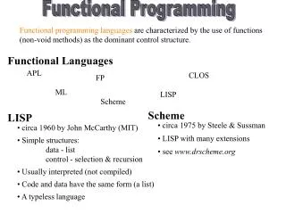
Language Families • Imperative (or Procedural, or Assignment-Based) • Functional (or Applicative) • Logic (or Declarative)
Imperative Languages • Mostly influenced by the von Neumann computer architecture • Variables model memory cells, can be assigned to, and act differently from mathematical variables • Destructive assignment, which mimics the movement of data from memory to CPU and back • Iteration as a means of repetition is faster than the more natural recursion, because instructions to be repeated are stored in adjacent memory cells
Functional Languages • Model of computation is the lambda calculus (of function application) • No variables or write-once variables • No destructive assignment • Program computes by applying a functional form to an argument • Program are built by composing simple functions into progressively more complicated ones • Recursion is the preferred means of repetition
Logic Languages • Model of computation is the Post production system • Write-once variables • Rule-based programming • Related to Horn logic, a subset of first-order logic • AND and OR non-determinism can be exploited in parallel execution • Almost unbelievably simple semantics • Prolog is a compromise language: not a pure logic language
What is a Functional Language? Opinions differ, and it is difficult to give a precise definition, but generally speaking: • Functional programming is style of programming in which the basic method of computation is the application of functions to arguments; • A functional language is one that supports and encourages the functional style.
Example Summing the integers 1 to 10 in Java: total = 0; for (i = 1; i 10; ++i) total = total+i; The computation method is variable assignment. 7
Example Summing the integers 1 to 10 in Haskell: sum [1..10] The computation method is function application. 8
Simple Function Definition • Examples from Sebesta fact 0 = 1 fact n = n * fact (n -1) fact1 = prod [1..n] fib 0 = 1 fib 1 = 1 fib (n + 2) = fib (n + 1) + fib n
Guards and otherwise fact n | n == 0 = 1 | n > 0 = n * fact (n – 1) • fact will not loop forever for a negative argument! sub n | n < 10 = 0 | n > 100 = 2 | otherwise = 1
Local scope: where quadratic_root a b c = [minus_b_over_2a – root_part_over_2a, minus_b_over_2a + root_part_over_2a] where minus_b_over_2a = -b / (2.0 * a) root_part_over_2a = sqrt(b ^ 2 – 4.0 * a * c) / (2.0 * a)
List comprehensions, generators, and tests • List comprehensions are used to define lists that represent sets, using a notation similar to traditional set notation: [body | qualifiers], e.g., [n * n * n | n <- [1..50]] defines a list of cubes of the numbers from 1 to 50 • Qualifiers can be generators (as above) or tests • The following function returns the list of factors of n factors n = [i | i <- [1 .. n div 2], n mod i == 0]
A Taste of Haskell f [] = [] f (x:xs) = f ys ++ [x] ++ f zs where ys = [a | a xs, a x] zs = [b | b xs, b > x] ? 13
Quicksort The quicksort algorithm for sorting a list of integers can be specified by the following two rules: • The empty list is already sorted; • Non-empty lists can be sorted by sorting the tail values the head, sorting the tail values the head, and then appending the resulting lists on either side of the head value.
Using recursion, this specification can be translated directly into an implementation: qsort :: [Int] [Int] qsort [] = [] qsort (x:xs) = qsort smaller ++ [x] ++ qsort larger where smaller = [a | a xs, a x] larger = [b | b xs, b x] Note: • This is probably the simplest implementation of quicksort in any programming language!
q [2,1] ++ [3] ++ q [4,5] q [1] ++ [2] ++ q [] q [] ++ [4] ++ q [5] [] [1] [] [5] For example (abbreviating qsort as q): q [3,2,4,1,5]
Lazy evaluation • Lazy evaluation allows infinite data structures, e.g.: positives = [0 ..] squares = [n * n | n <- [0..]] • member squares 16 • member [] b = False member (a:x) b = (a == b) || member x b • member2 (m:x) n | m < n = member2 x n | m == n true otherwise = False