Boundary Layer Flow
Boundary Layer Flow. p < 0. t w. U. U. p > 0. Drag force. The surrounding fluid exerts pressure forces and viscous forces on an object . The components of the resultant force acting on the object immersed in the fluid are the drag force and the lift force. . p < 0. t w. U. U.


Boundary Layer Flow
E N D
Presentation Transcript
p < 0 tw U U p > 0 Drag force • The surrounding fluid exerts pressure forces and viscous forces on an object. • The components of the resultant force acting on the object immersed in the fluid are the drag force and the lift force.
p < 0 tw U U p > 0 Drag prediction • The drag force is due to the pressure and shear forces acting on the surface of the object. • The tangential shear stresses acting on the object produce friction drag (or viscous drag).
p < 0 tw U U p > 0 Drag prediction • Friction drag is dominant in flow past a flat plate and is given by the surface shear stress times the area: • Pressure or form drag results from variations in the normal pressure around the object:
Viscous boundary layer • An originally laminar flow is affected by the presence of the walls. • Flow over flat plate is visualized by introducing bubbles that follow the local fluid velocity. • Most of the flow is unaffected by the presence of the plate.
Viscous boundary layer • However, in the region closest to the wall, the velocity decreases to zero. • The flow away from the walls can be treated as inviscid, and can sometimes be approximated as potential flow.
Viscous boundary layer • The region near the wall where the viscous forces are of the same order as the inertial forces is termed the boundary layer.
Viscous boundary layer • The distance over which the viscous forces have an effect is termed the boundary layer thickness. • The thickness is a function of the ratio between the inertial forces and the viscous forces- i.e., the Reynolds number. As NReincreases, the thickness decreases.
Effect of viscosity • The layers closer to the wall start moving right away due to the no-slip boundary condition. The layers farther away from the wall start moving later. • The distance from the wall that is affected by the motion is also called the viscous diffusion length. This distance increases as time goes on.
Moving plate boundary layer • Consider an impulsively started plate in a stagnant fluid. • When the wall in contact with the still fluid suddenly starts to move, the layers of fluid close to the wall are dragged along while the layers farther away from the wall move with a lower velocity. • The viscous layer develops as a result of the no-slip boundary condition at the wall.
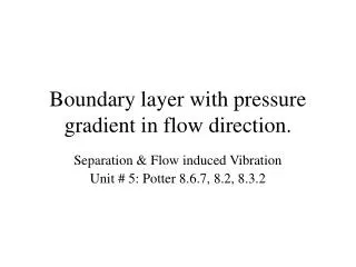
Flow separation Flow separation occurs when (a) the velocity at the wall is zero or negative and an inflection point exists in the velocity profile, and a positive or adverse pressure gradient occurs in the direction of flow.
Boundary layer theory • Consider a flow over a semi-infinite flat plate (and also for a finite flat plate), under steady state conditions: Fluid Velocity, v • Away from plate, inviscidflow assumption is valid. • Near the plate, viscosity effects are significant.
Velocity v INF INF INVISCID FLOWASSUMPTION OK HERE Velocity v No Slip FRICTION CANNOT BENEGLECTED HERE Velocity 0 0 0 Boundary layer theory Solid Boundary
INF INF d d 0 0 Boundary layer theory Solid Boundary BL thickness 99% Free stream velocity What happens to d when you move in x? BL thickness increases with x x
Laminar boundary layer BL Reynolds number: Blasius approximation of d:
Turbulent boundary layer At high enough fluid velocity, inertial forces dominate • Viscous forces cannot prevent a wayward particle from motion • Chaotic flow ensues Turbulence near the wall • For wall-bounded flows, turbulence initiates near the wall
Turbulent boundary layer • In turbulent flow, the velocity component normal to the surface is much smaller than the velocity parallel to the surface • The gradients of the flow across the layer are much greater than the gradients in the flow direction.
Turbulent boundary layer Eddies and Vorticity • An eddy is a particle of vorticity that typically forms within regions of velocity gradient • An eddy begins as a disturbance near the wall, followed by the formation of a vortex filament that later stretches into a horseshoe or hairpin vortex
Turbulent boundary layer • Turbulence is comprised of irregular, chaotic, three-dimensional fluid motion, but containing coherent structures. • Turbulence occurs at high Reynolds numbers, where instabilities give way to chaotic motion. • Turbulence is comprised of many scales of eddies, which dissipate energy and momentum through a series of scale ranges. The largest eddies contain the bulk of the kinetic energy, and break up by inertial forces. The smallest eddies contain the bulk of the vorticity, and dissipate by viscosity into heat. • Turbulent flows are not only dissipative, but also dispersive through the advection mechanism.
Buckingham Pi Theorem • Tells how many dimensionless groups (p) may define a system. • Theorem: If n variables are involved in a problem and these are expressed using kbase dimensions, then (n – k) dimensionless groups are required to characterize the system/problem.
Buckingham Pi Theorem Example: In describing the motion of a pendulum, the variables are time [T], length [L], gravity [L/T2], mass [M]. Therefore, n= 4 k= 3. So, only one (4 – 3) dimensionless group is required to describe the system. But how do we derive this?
Buckingham Pi Theorem How to find the dimensional groups: For the pendulum example: let a, b, c and dbe the coefficients of t, L, g and m in the group, respectively. In terms of dimensions:
Buckingham Pi Theorem How to find the dimensional groups: For the pendulum example: let a, b, c and d be the coefficients of t, L, g and m in the group, respectively. Since the group is dimensionless: Therefore:
Buckingham Pi Theorem How to find the dimensional groups: For the pendulum example: let a, b, c and d be the coefficients of t, L, g and m in the group, respectively. Arbitrarily choosing a =1: Therefore:
Buckingham Pi Theorem Example: Drag on a sphere • Drag depends on FOUR parameters: sphere size (D); fluid speed (v); fluid density (r); fluid viscosity (m) • Difficult to know how to set up experiments to determine dependencies and how to present results (four graphs?)
Buckingham Pi Theorem Step 1: List all the parameters involved Let n be the number of parameters Example: For drag on a sphere: F, v, D, r, and m (n= 5) Step 2: Select a set of primary dimensions Let kbe the number of primary dimensions For this example: M (kg), L (m), t (sec); thus k = 3
Buckingham Pi Theorem Step 3: Determine the number of dimensionless groups required to define the system Step 4: Select a set of kdimensional parameters that includes all the primary dimensions For example: select r, v, D
Buckingham Pi Theorem Step 4: Select a set of kdimensional parameters that includes all the primary dimensions For example: select r, v, D AND F
Buckingham Pi Theorem Step 4: Select a set of kdimensional parameters that includes all the primary dimensions For example: select r, v, D AND F Let d= 1: Therefore:
Buckingham Pi Theorem Step 4: Select a set of kdimensional parameters that includes all the primary dimensions Next group: select r, v, D andm
Buckingham Pi Theorem Step 4: Select a set of kdimensional parameters that includes all the primary dimensions Next group: select r, v, D andm Let a = 1: Therefore: