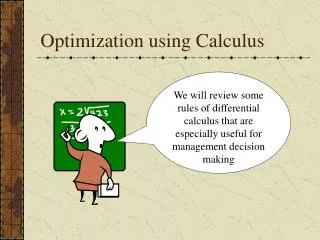
Optimization using Calculus
Optimization using Calculus. We will review some rules of differential calculus that are especially useful for management decision making. The profit function. Suppose that a business firm has estimated its profit ( ) function (based on marketing and production studies) as follows:.


Optimization using Calculus
E N D
Presentation Transcript
Optimization using Calculus We will review some rules of differential calculus that are especially useful for management decision making
The profit function Suppose that a business firm has estimated its profit () function (based on marketing and production studies) as follows: Where is profit (in thousands of dollars) and Q is quantity (in thousands of units). Thus the problem for management is to set its quantity(Q) at the level that maximizes profits ().
What is an objective function? The profit function shows the relationship between the manager’s decision variable (Q) and her objective (). That is why we call it the objective function.
The profit function again Marginal profit at a particular output is given by the slope of a line tangent to the profit function
Computing profit at various output levels using a spreadsheet • Recall our profit function is given by: = 2Q - .1Q2 – 3.6 • Fill in the “quantity” column with 0, 2, 4, . . . • Assume that you typed zero in column cell a3 of your spreadsheet • Place your cursor in the the cell b3 (it now contains the bolded number –3.6)—just to the right of cell a3. • Type the following in the formula bar:=(2*a3)-(.1*a3^2)-3.6and click on the check mark to the left of the formula bar. • Now move your cursor to the southeast corner of cell b3 until you see a small cross (+).Now move your cursor down through cells b4, b5, b6 . . . to compute profit at various levels of output.
Rules of calculus Rule 1: The derivative of a constant is zero. y Example: Let Y = 7 Thus: dy/dx = 0 7 0 X
Rule 2 Rule 2: The derivative of a constant times a variable is simply the constant. y Example: Let y = 13x Thus: dy/dx = 13 26 13 0 1 2 x
Rule 3 Rule 3: A power function has the form y = axn, where a and n are constants. The derivative of a power function is: Example: Let y = 4x3Thus: dy/dx= 12x2
Power functions Special cases of the power function • Note the following: • y =1/x2 is equivalently written as y = x-2and can be written y = x1/2 Hence by rule 3 (or the power rule), the respective derivatives are given by: dy/dx = -2x-3 And dy/dx = .5x-1/2 =
Rule 4 Rule 4: Suppose the product of two functions : y = f(x)g(x). Then we have: Example: Let y = (4x)(3x2) Thus: dy/dx = (4)(3x2) + (4x)(6x) = 36x2
Rule 5 Rule 5: The derivative of the sum of functions is equal to the sum of the derivatives. If y = f(x) + g(x), then: dy/dx = df/dx + dg/dx Example: Let: y = .1x2 – 2x3 Thus: dy/dx = .2x – 6x2
Rule 6 Rule 6: Suppose y is a quotient: y = f(x)/g(x). Then we have: Example Suppose we have: y = x/(8 + x) Thus: dy/dx = [1 • (8 + x) – 1 • (x)]/ (8 + x)2 = 8/(8 + x)2
The marginal profit (M) function Let the profit function be given by: = 2Q - .1Q2 – 3.6 To obtain the marginal profit function, we take the first derivative of profit with respect to output (Q): M = d/dQ = 2 - .2Q To solve for the output level that maximizes profits, set M =0. 2 - .2Q = 0 Thus: Q = 10
The second derivative We know that the slope of the profit function is zero at its maximum point. So the first derivative of the profit function with respect to Q will be zero at that output. Problem is, how do we know we have a maximum instead of a minimum?
Notice this function has a slope of zero at two levels of output A more complicated profit function
Taking the second derivative Our profit function () is given by: Now let’s derive the marginal profit (M )function We can verify that M = 0 when Q = 2 and Q = 10.
Maximum or minimum? Notice at the minimum point of the function, the slope is turning from zero to positive. Notice also at the maximum point, the slope is changing from zero to negative
To insure a maximum, check to see that the second derivative is negative To take the second derivative of the profit function: Thus we have: Hence, when Q = 2, we find that d2/dQ2 = 3.6 - .6(2) = 2.4 When Q = 10, we find that d2/dQ2 = 3.6 - .6(10) = -2.4
Marginal Revenue and Marginal Cost MR = MC Marginal profit (M) is zero when marginal revenue (MR) is equal to marginal cost (MC), or alternatively, when MR – MC = 0. Hence to find the profit maximizing output, set the first derivative of the revenue function equal to the first derivative of the cost functions
Solving for the profit maximizing output Let (Q) = R(Q) – C(Q),where R is sales revenue and C is cost Thus we have
Multivariable functions y = f(x, z, w) Suppose we have a multivariate function such as the following: = f(P, A), where P is market price and A is the advertising budget. Our function has been estimated as follows: • We would like to know: • How sensitive are profits to a change in price, other things being equal (or ceteris paribus)? • How sensitive are profits to a change in the advertising budget, ceteris paribus?
We get the answer to question 1 by taking the first partial derivative of with respect to P. Partial derivatives We can find the answer to question 2 by taking the first partial derivative of with respect to A:
Solving for the P and A that maximize We know that profits will be maximized when the first partial derivatives are equal to zero. Hence, we set them equal to zero and obtain a linear equation system with 2 unknowns (P and A) 2 – 4P + 2A= 0 4 - 2A + 2P = 0 The solution is:P = 3 and A = 5
Constrained optimization So far we have looked at problems in which the decision maker maximizes some variable () but faces no constraints. We call this “unconstrained optimization.” Often, however, we seek to maximize (or minimize) some variable subject to one or constraints. • Examples: • Maximize profits subject to the constraint that output is equal to or greater than some minimum level. • Maximize output subject to the constraint that cost must be equal to or less than some maximum value.
Example 1 Suppose we are seeking to maximize the following profit function subject to the constraint that Q 7. What happens if we take the first derivative, set equal to zero, and solve for Q? Solving to maximize , we get Q = 5. But that violates our constraint.
Another example A firm has a limited amount of output and must decide what quantities (Q1 and Q2) to sell in two different market segments. Suppose its profit () function is given by: The firm’s output cannot exceed 25—that is, it seeks to maximize subject to Q 25. If we set the marginal profit functions equal to zero and solved for Q1 and Q2, we would get: Q1 = 20 and Q2 = 20, so that Q1 + Q2 =40. Again, this violates the constraint that total output cannot exceed 25.
Method of Lagrange Multipliers This technique entails creating a new variable (the Lagrange multiplier) or each constraint. We then determine optimal values for each decision variable and the Lagrange multiplier.
Lagrange technique: Example 1 Recall example 1 . Our constraint was given by Q = 7. We can restate this constraint as: 7 – Q = 0 Our new variable will be denoted by z. Our Lagrange (L) function can be written:
Taking the partials of L with respect to Q and z Now we just take the first partial derivative of Lwith respect to Q and z, set them equal to zero, and solve. Solving for Q and z simultaneously, we obtain: Q = 7 and z = -16
Interpretation of the Lagrange multiplier (z) You may interpret the result that z = -16 as follows: marginal profit (M) at the constrained optimum output is –16 —that is, the last unit produced subtracted $16 for our profit
Lagrange technique: Example 2 Recall example 2 . Our constraint was given by: Q1 + Q2 = 25 Our Lagrange (L) function can be written as :
Taking the partials of L with respect to Q1, Q2 and z This time we take the first partial derivative of Lwith respect to Q1, Q2, and z, set them equal to zero, and solve. The solutions are:Q1 = 10Q2 = 15z = 10