Download
1 / 23
280 likes | 868 Vues
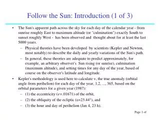
Follow the Sun: Introduction (1 of 3). The Sun's apparent path across the sky for each day of the calendar year - from sunrise roughly East to maximum altitude (or "culmination") exactly South to sunset roughly West - has been observed and thought about for at least the last 5000 years.

E N D
Follow the Sun: Introduction (1 of 3) The Sun's apparent path across the sky for each day of the calendar year - from sunrise roughly East to maximum altitude (or "culmination") exactly South to sunset roughly West - has been observed and thought about for at least the last 5000 years. Physical theories have been developed by scientists (Kepler and Newton, most notably) to describe the daily and yearly variations of the Sun's path. In general, these theories are adequate to predict approximately, for example, an arbitrary observer's Sun rising (or sunrise), culmination (maximum altitude), and setting times for any day of the year, based of course on the observer's latitude and longitude. Kepler's methodology is used here to calculate , the true anomaly (orbital angle from perihelion) for each day of the year, 1,2, ..., 365, based on the orbital parameters for a given year (1987): (1) the eccentricity (e=.01671) of the orbit, (2) the obliquity of the ecliptic (=23.44), and (3) the hour and day of perihelion (Jan 4, 23 h). Page 1 of
Follow the Sun: Introduction (2 of 3) Kepler's method is used to calculate , the true anomaly (orbital angle from perihelion) - angle along the cyan curve - based on the orbital parameters for a given year (1987): the eccentricity (e=.016712) of the orbit, and the obliquity of the ecliptic (=23.45). Angle is measured from perihelion - angle along the cyan curve - as measured at the Greenwich meridian. For 1987, for example, the perihelion occurred on the 23rd hour of January 4th, or more briefly as Jan 4 23h. Jan 1 Page 2 of
Follow the Sun: Introduction (3 of 3) Suppose the Sun is at a given position at a certain time, Jan 1, 1987. The Sun will take from this point one of 2 "paths" on the Celestial Sphere, based entirely on the measurement period employed: (1) record once every (solar day) T = 24 hours to produce points on (and ultimately all) the red curve (2) record once every (sidereal day) TE = 23h 56m 4.091 s to produce points on (and ultimately all) the cyan curve N equator ecliptic Jan1 Page 3 of
Kepler's Analysis of Planetary Motion • Kepler proposed a model for planetary motion - with solid empirical evidence for his pronouncements from his study of astronomer Tycho Brahe's (16th century) observations of the planets. His Laws can be stated as [1] • (1) The orbit of each planet is an ellipse, and the Sun (at S in the upcoming drawings) is at a focus of that ellipse. • (2) The line joining Sun (S) and planet (Q) sweeps out equal areas in equal times. • (3) The square of the period of revolution (Tyear) of the planet is proportional to the cube of its mean distance from the Sun. • We assume the 3 Laws are true - at least for the accuracy needed - and follow Kepler in analyzing for the position in the elliptical orbit as a function of time. • Due to symmetry it is convenient to measure time t from perihelion (the closest point in the orbit of a Planet to the Sun), which we denote by t0. • The next slide depicts an orbit with a moderately large eccentricity (e) of 0.55. [1] Fundamentals of Astrodynamics, Bate, Mueller, and White, Dover (1971)
Elliptical Orbit: Anomaly Illustration, Example 1 • A blue ellipse is drawn with center point O. The semimajor axisa is 1 unit, and b is the semiminor axis. Here the ellipticity e is about 0.55. • The black dot labeled S (at the focus of the ellipse) represents the Sun; P the perihelion point is in the orbit along ray OS. The time t0 at perihelion is given. • The auxiliary red circle about O has radius a and contains P. • Q is the planet at time t; Q' is the (nearer) point on the circle at the same distance as Q from a perpendicular to OS. Q' b Q E P O S a = |OP|
Elliptical Orbit: Anomaly Illustration, Example 1 • As the planet progresses through the orbit the true anomaly angle increases monotonically from 0 degrees at perihelion to 180 degrees at aphelion, the farthest the Planet is from the Sun. • After aphelion, and up until the next passage of the perihelion point, increases (again monotonically) from 180 to 360. • We note that • (1) E < for 0 < < 180 • (2) E > for 180 < < 360. • We consider a last example for Q past aphelion on the next slide. Q' Q Q' Q E E O S P P O S
Elliptical Orbit: Anomaly Illustration, Example 1 • A third position in the orbit illustrates a case with E and between 180 and 360 degrees. • Again Q is the point along the orbit, and Q' is on the auxiliary circle, and at the same distance as Q from a perpendicular to the semimajor axis. • By symmetry we note that any problem with > 180 has an identical trignometric problem with ' = 360 - . • For 0 < < 180 we choose Q' above the semimajor axis OP, and Q' below the semimajor axis for 180 < < 360. E O P S Q Q'
Eccentric Anomaly as a Function of Time t in the Elliptical Orbit (1 of 3) • We look for A(t), the area swept out in time t by the radius vector (SQ) from perihelion. • Circular sector Q'OP has an area proportional to E. With E in degrees we have Q' b Q E P O S a = |OP| • The ratio of the area of elliptical sector QOP to the area of circular sector Q'OP is equal to the aspect ratio (b/a) of the ellipse:
Eccentric Anomaly as a Function of Time t in the Elliptical Orbit (2 of 3) • The area A(t) of elliptical sector QSP (centered on S) in (3) is the difference of the area of sector QOP (centered on O) and triangle QOS. Q' b Q E P O S a = |OP|
Eccentric Anomaly as a Function of Time t in the Elliptical Orbit (3 of 3) • By equal areas in equal times, the time from perihelion to the period Tyear equals the ratio of the area of sector QSP to the area of the ellipse: Q' b Q E P O S a = |OP|
Solving Kepler's Equation • Solving Kepler's Equation means finding Ethat satisfies (5) given eccentricity e, time of perihelion t0, and t. • A simple Newton-Raphson root-finding approach was found to converge rapidly, at least for the eccentricities (.0167 and .55) considered. Define from (5) a function of E that we can adjust in E to make f(E) = 0. • The following equation can be iterated to determine a new value of E (in degrees) from a tentative value, given eccentricity e (unitless) and M (in degrees).
True Anomaly from Eccentric Anomaly • We can relate E and by simple trigonometry. Q' y Q E P O S x • We see from these relations that the tangent of is related to E and e.
True, Eccentric, and Mean Anomaly for b/a = 5/6, e = 0.55277 • The true, mean, and eccentric anomalies are plotted for a very eccentric orbit, e 0.55. • The green curve is a straight line, and is subtracted from the other curves below.
True, Eccentric, and Mean Anomaly for b/a = .99986, e = 0.01671 (Earth for 1987) e = 0.0167 • For the Earth, the absolute difference between true and mean anomaly is never more than 2 degrees. The orbit pictured previously shows +/- 60 degrees of variation. e = 0.553
AnomalyVariation Around March Equinox and Summer Solstice • Around the March Equinox (during day 80 or March 21st) is about 2 degrees greater than M, whereas at the Summer Solstice (during day 173 or June 22nd) is about 1/2 of a degree:
Sun's Yearly Path on the Celestial Sphere A plot of the Sun's apparent path (at 24 hour intervals) throughout the entire year along the celestial sphere is shown as a red line. A cyan asterisk marks Jan 1st on the red "figure 8". The curve crosses the Equator (blue circle) in March, and reaches its highest angle (declination = 23.45) in June (around Jun 21). The Sun follows the 8 to cross the Equator for a second time (going South) in September, reaching the "low point" (declination = -23.45) in December (around Dec 22nd.) The cycle then repeats, with a slightly different starting point. Page 16 of 37
Ecliptic and Celestial Equator The (celestial) equator is the blue arc in the figure, 90 degrees from point N, (the Celestial North pole), indicated as a blue dot. A cyan great circle is a depiction of the ecliptic, the observed path of the Sun against the fixed stars, assuming that the Sun is at the asterisk on Jan 1st. The restrictions on the cyan great circle are that it (1) go through the initial (Jan 1) point, and (2) intersect the Equator at and angle of = 23.45 N equator ecliptic Jan1 Page 17 of 37
Starting out in January, first 5 days A cyan asterisk is used to show the initial position of the Sun, for example, January 1st. Along the red curve is the analemma path, sampled at 2 week intervals. The cyan symbols mark points along the ecliptic. close up Jan29 Nov 19 Jan15 Jan1 Dec 3 Dec 17 Page 18 of 37
Finding the "Jan 2" Point on the Analemma A "two-step" procedure generates the Jan 2 analemma position, the green dot in the closeup view. first step along ecliptic second step back along declination circle Nov5 Jan31 closeup Nov19 Jan15 Dec3 Jan15 Dec31 \ Jan 1 Dec17 Dec31 Dec17 Jan1 Page 19 of 37
Finding the 2nd Point on the Analemma The first step is along the ecliptic, the cyan arc, from the initial point to B. The length of the step is determined from the true anomaly variation for Jan 1, 1987, about 1.01924 degrees/day. The second step is back to 2 along the declination circle of B. The length of the 2nd step is a multiple of a fixed angle: the rotation rate of the Earth times the difference between the solar and sidereal day, or 0.985645401 degrees. B 2 1 Page 20 of 37
Constructing the Positional Coordinates of the Sun • We repeat the process of generating a next point on the analemma from a given point over and over again. • The magenta points are the calculated analemma positions of the Sun at 7 day intervals in 1987. • The red squares are the positions given in the 1987 almanac for the Sun's declination and meridian. • The red squares are the listed values in the Almanac, and at 15 day intervals (extending between Jan 1 and Dec 31).
Finding the 3rd Point The third point is found as follows. The first step is from B along the ecliptic to C, a distance proportional to the daily change in true anomaly on Jan 2 (1.01926) The second step is back along C's declination circle, but this arc is twice as long as before. We reason that C is 2 rotations of the Earth later, so two "time corrections"are needed to adjust to 2 solar days after Jan 1. Jan 15 3 2 C B Jan 1 Page 22 of 37
First 5 Points The 4th and 5th point are found similarly Another point is added (Jan 8) to the red curve. Jan 29 Jan 15 5 Jan 8 3 E C Jan 1 Page 23 of 37