Accretion-ejection and magnetic star-disk interaction: a numerical perspective
350 likes | 488 Vues
This presentation explores the dynamics of accretion-ejection mechanisms in astrophysical contexts, focusing on magnetically controlled accretion processes and the roles of disk winds and stellar winds. Observational evidence supporting these scenarios is discussed alongside the advantages and limitations of analytical models versus numerical simulations. The magneto-centrifugal mechanism is highlighted, detailing how magnetic fields influence outflows from young stellar objects (YSOs). Emphasis is placed on the importance of large-scale magnetic fields and the implications for understanding star formation and disk evolution.

Accretion-ejection and magnetic star-disk interaction: a numerical perspective
E N D
Presentation Transcript
Accretion-ejection and magnetic star-disk interaction: a numerical perspective Claudio Zanni Laboratoire d’Astrophysique de Grenoble 5th JETSET School January 8th – 12th 2008 Galway - Ireland
Outline • Observational evidences supporting these scenarios: • - accretion-ejection (disk-winds) (45 min) • - magnetically controlled accretion (45 min) • What analytical models can do? • - pros: exact solutions, analysis of the parameter space • - cons: stationarity, self-similarity • What numerical simulations can do? • - pros: time-dependent, no self-similarity, 3D • - cons: can you trust them?
Ejection: jets from YSO • They are directly observed ! • - dynamics (speed, rotation) • - thermodynamics (temperature, • chemistry) • … but not close enough to the • central source to give direct • informations on their origin
Proposed scenarios Extended disk wind X-wind Stellar wind • Succesful models require large-scale magnetic fields with • plasma flowing along the magnetic surfaces: • -extended disk wind: Bz distributed on a large radial extension • -X-wind: Bz exists only in a tiny region around the magnetopause • -stellar wind: opened magnetic field anchored on the star
Why extended disk winds are important ? Ferreira, Dougados, Cabrit (2006) For a given footpoint r0 relation between toroidal and poloidal speed: • Extended disc winds, X-winds, and stellar winds occupy distinct regions in the plane Only extended disk winds give results consistent with observations
Ejection: how it works?The magneto-centrifugal mechanism • At Alfven surface matter inertia • bends the lines and field gets • wound up • Toroidal magnetic field controls • collimation (magnetic “hoop • stress”) and pushes the outflow • Magnetic field lines frozen in a disk • rotating at Keplerian rate k • “Bead on the wire” accelerated with • constant k if fieldline is open • > 60o • Angular momentum extraction • accretion
Framework: MHD • Conservation of: • Mass • Momentum • Energy • Induction equation: with • Solenoidality of the field:
Assumptions: • - stationarity • - axisymmetry • - self-similarity (Radially self-similar solution) Analytical solutions (1) • Invariants: • Specific angular momentum • (lever arm) • Mass loading • Field angular velocity • Entropy • Energy (Bernoulli equation)
Analytical solutions (2) • An entire class of radially self-similar • MHD solutions can be constructed • (Vlahakis et al. 1998, see Rammos’ poster) • Examples (Contopoulos & Lovelace 1994): Bz/ r -1.2 Bz/ r -0.98 Bz/ r -1.1 • Blandford & Payne (1982) • - Trans-Alfvenic solution • - Bz/ r -5/4
Numerical solutions • Why time-dependent simulations? • - Test the analytical models • - Go beyond self-similarity • - time-dependent variability • - 3D models – stability • - combine different components (stellar wind)
Ejection: initial conditions Keplerian rotation + injection boundary Initial analytical solution (one ore more superposed) + boundary conditions (Gracia et al. 2006, Matsakos et al. 2008, and see Stute’s poster) B) A) Boundary conditions (rotation/injection) + non-rotating magnetized corona (Ouyed & Pudritz 1997)
Ejection: boundary conditions • Injection boundary: number of incoming characteristics = number of fixed • variables. Other variables must be free to evolve. • Outer boundaries: even if the flow is • super-fastmagnetosonic, pay attention • at the direction of the Mach cones • ( below or beyond the separatrix) Example: “outflow” condition on B at rout Artificial collimating effect Ustyugova et al. (1999)
Testing stationary models (1) • Axisymmetric MHD invariants • are almost constant Ustyugova et al. (1999) Ustyugova et al. (1999) • Acceleration mechanism IS • magneto-centrifugal: dominant • forces are centrifugal (C) and • Lorentz (M)
Testing stationary models (2) • MHD invariants Matsakos et al. (2008) Matsakos et al. (2008) • Wave-structure and • characteristic surfaces of • analytical solutions are • recovered
Non-stationarity / variability • When the outflow is too • mass-loaded, the flow • “lags behind” the • Keplerian rotation and falls • towards the center • (Anderson et al. 2004) 1) • “Overdetermined” • boundary conditions • force the propagation of • MHD shocks along the jet • (Ouyed & Pudritz 1997b) 2)
3D simulations • Some technical issues: • How to put a circle inside a • square: smoothly reduce the • rotation to zero between r0 and rmax • Ensure r v = 0 and r B = 0 in • the injection boundary Ouyed, Clarke & Pudritz (2003)
3D simulations – stability (1) • “Corescrew” or wobbling solutions are • found which are not destroyed by the • non-axisymmetric (m=1) modes • A self-regulatory mechanism is found • which maintains the flow sub-Alfvenic • and therefore more stable (Ray 1981, • Hardee & Rosen 1999) Ouyed, Clarke & Pudritz (2003)
3D simulations – stability (2) • Asymmetric outflow stabilized by • a (light) fast- moving outflow • near the axis with a poloidally • dominated magnetic field. Anderson et al. (2006)
… what about accretion? • Additional elements must be taken into account … • - Accretion (mass conservation) • - Disk vertical equilibrium (mass loading) • - Field diffusion
… what about accretion? • Mass conservation: : ejection efficiency • Disk vertical equilibrium: Only thermal pressure can uplift matter at the disk surface • Magnetic field diffusion: Diffusion must counteract advection of the footpoints of the fieldlines
Analytical self-similar solutions Radially self-similar solution now depends on the disk parameters: magnetization disk thickness Ferreira (1997) magnetic diffusion • Important results: • - jet parameter space strongly reduced • - field must be around equipartition (» 1) and m» 1 (or strongly anisotropic)
What simulations can do? Zanni et al. (2007) Casse & Keppens (2004) … And give a look to Tzeferacos’ poster
Initial-boundary conditions Self-similar Keplerian disk in equilibrium with gravity, pressure gradients and Lorentz forces. Disk parameters: Resolution: FLASH – AMR / 7 levels of refinement / 512x1536 eq. resolution
Resistivity parameter m = 1 Smooth, trans-Alfvenic, trans-fastmagnetosonic outflow is accelerated
Mass loading - acceleration P G M • Lorentz toroidal force changes • sign at the disk surface • Magnetic field extracts angolar • momentum from the disk and • transfer to the outflow • Thermal pressure gradients supports • the disk against gravity and magnetic • pinch • Pressure provides the mass loading • and then Lorentz forces accelerate • the outflow
Current circuits - collimation Lorentz force (JxB) perpendicular to electric current circuits (rB = const) Outflow collimated only towards the axis. Outer part still uncollimated Zanni et al. (2007) Ferreira (1997)
Axisymmetric MHD invariants r0 = 2 r0 = 8 r0 = 4 r0 = 4 r0 = 2 r0 = 8 Flow perpendicular to the fieldlines in the disk and parallel in the jet (resistive – ideal MHD transition) Weber & Davis (1967) Inner fieldlines more stationary Radial dependency of and k
Resistivity parameter m = 0.1 Footpoints of the fieldline advected towards the central object Differential rotation along the fieldlines triggers a “magnetic tower”
Parameter study - diagnostics Increasing m Increasing m • Ejection efficiencies consistent • with observations (Cabrit 2002) • Terminal speeds around 1-2 times • the escape velocity ! Simulated spatial scale too small to check rotation ! But » 9 in the outer fieldlines of the outflow (see Ferreira et al. 2006)
Is everything ok? Despite having the same disk parameters (» 0.6, m» 1, » 0.1), analytical and numerical solutions have different jet parameters Numerical: - k » 0.1 - 0.3 -» 4 - 9 -» 0.09 Analytical: - k » 2£ 10-2 -» 35 -» 0.01 Analytical solution less mass loaded and faster ( )
A physical reason Zanni et al. (2007) Casse & Keppens (2004) • No analytical trans-Alfvenic solutions found when the electric current • enters the surface of the disk (mass loading too high) • Inner boundary forces the current to enter at the surface of the disk in • its inner radii. The mass outflow is strongly enhanced in this region
A numerical reason Casse & Ferreira (2000) • Density jump at the disk surface • under-resolved in current • simulations • Numerical solutions closer to • “warm” analytical models. • Dissipation at the disk surface • With a resolution 4 times lower it is • possible to find stationary solutions • even with m» 0.1 • Radial numerical diffusion of Bz
Perspectives • Parameter space analysis • - Magnetization (see Tzeferacos’ poster) • - Transition between jet emitting and non-emitting • disks (standard accretion disk) • - The missing link between the small and the large scale • - Interaction with an inner component (Meliani et al. 2006) • Go to 3D …