spike-triggering stimulus features

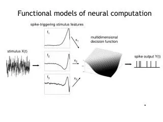
1. Functional models of neural computation spike-triggering stimulus features f1 multidimensional decision function x1 stimulus X(t) f2 spike output Y(t) x2 f3 x3

2. Given a set of data, want to find the best reduced dimensional description. The data are the set of stimuli that lead up to a spike, Sn(t) , where t = 1, 2, 3, …., D Variance of a random variable = < (X-mean(X))2> Covariance = < (X – mean(X))T (X – mean(X)) > Compute the difference matrix between covariance matrix of the spike-triggered stimuli and that of all stimuli Find its eigensystem to define the dimensions of interest

3. Eigensystem: any matrix M can be decomposed as M = U V UT , where U is an orthogonal matrix; V is a diagonal matrix, diag([l1,l2,..,lD]). Each eigenvalue has a corresponding eigenvector, the orthogonal columns of U. The value of the eigenvalue classifies the eigenvectors as belonging to column space = orthogonal basis for relevant dimensions null space = orthogonal basis for irrelevant dimensions We will project the stimuli into the column space.

4. This method finds an orthogonal basis in which to describe the data, and ranks each “axis” according to its importance in capturing the data. Related to principal component analysis.

5. Example: An auditory neuron is responsible for detecting sound at a certain frequency w. Phase is not important. The appropriate “directions” describing this neuron’s relevant feature space are Cos(wt) and Sin(wt). This will describe any signal at that frequency, independent of phase: cos(A+B) = cos(A) cos(B) - sin(A) sin(B)  cos(wt + f) = a cos(wt) + b sin(wt), a = cos(f), b = -sin(f). Note that a2 + b2 = 1; all such stimuli lie on a ring.

6. 0.4 0.3 0.2 0.1 Velocity 0 -0.1 -0.2 -0.3 -0.4 150 100 50 0 Pre-spike time (ms) Modes look like local frequency detectors, in conjugate pairs (sin & cosine)… and they sum in quadrature, i.e. the decision function depends only on x2 + y2

7. Basic types of computation: • integrators (H1) • differentiators (retina, simple cells, single neurons) • power detectors (complex cells, somatosensory, auditory, • retina)

8. Decoding How well can we learn what the stimulus is by looking at the neural responses? Two approaches: devise explicit algorithms for extracting a stimulus estimate directly quantify the relationship between stimulus and response using information theory

9. Motion detection task: two-state forced choice Britten et al.: behavioral monkey data + neural responses

10. Behavioral performance Neural data at different coherences Discriminability: d’ = ( <r>+ - <r>- )/ sr

11. z p(r|-) p(r|+) <r>+ <r>- Signal detection theory: r is the “test”. a(z) = P[ r>= z|-] false alarm rate, “size” b(z) = P[ r>= z|+] hit rate, “power” Could maximize P[correct] = (b(z) + 1 – a(z))/2

12. ROC curves: summarize performance of test for different thresholds z Want b 1, a  0.

13. The area under the ROC curve corresponds to P[correct] for a two-alternative forced choice task: first presentation acts as threshold for second. If p[r|+] and p[r|-] are both Gaussian, P[correct] = ½ erfc(-d’/2). Ideal observer: performs as area under ROC curve.

14. Close correspondence between neural and behaviour.. Why so many neurons? Correlations limit performance.

15. What is the best test function to use? (other than r) Neyman-Pearson lemma: the optimal test function is the likelihood ratio, l(r) = p[r|+] / p[r|-]. Note that l(z) = (db/dz) / (da/dz) = db/da