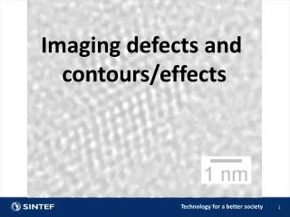
Imaging defects and contours/effects
Imaging defects and contours/effects. Dynamical diffraction theory. Dynamical diffraction: A beam which is diffracted once will easily be re-diffracted (many times..). Understanding diffraction contrast in the TEM image.

Imaging defects and contours/effects
E N D
Presentation Transcript
Imaging defects and contours/effects
Dynamical diffraction theory Dynamical diffraction: A beam which is diffracted once will easily be re-diffracted (many times..) Understanding diffraction contrast in the TEM image In general, the analysis of the intensity of diffracted beams in the TEM is not simple because a beam which is diffracted once will easily be re-diffracted. We call this repeated diffraction ‘dynamical diffraction.’
Dynamical diffraction: Assumption: That each individual diffraction/interference event, from whatever locality within the crystal, acts independently of the others Multiple diffraction throughout the crystal; all of these waves can then interfere with each other Ewald: Diffraction intensity, I, is proportional to just the magnitude of the structure factor, F, is referred to as the dynamical theory of diffraction We cannot use the intensities of spots in electron DPs (except under very special conditions such as CBED) for structure determination, in the way that we use intensities in X-ray patterns. Ex. the intensity of the electron beam varies strongly as the thickness of the specimen changes http://pd.chem.ucl.ac.uk/pdnn/diff2/kinemat1.htm
THE AMPLITUDE OF A DIFFRACTED BEAM The amplitude of the electron beam scattered from a unit cell is: Structure factor The intensity at some point P, we then sum over all the unit cells in the specimen. The amplitude in a diffracted beam: (rndenotes the position of each unit cell)
If the amplitude φgchanges by a small increment as the beam passes through a thin slice of material which is dz thick we can write down expressions for the changes in φ g and f0by using the concept introduced in equation 13.3 but replacing a by the short distance dz Two beam approximation Here χO-χDis the change in wave vector as the φg beam scatters into the φ0 beam. Similarly χD-χOis the change in wave vector as the φ0beam scatters into the φg beam. Now the difference χO-χDis identical to kOkDalthough the individual terms are not equal. Then remember that kDkO (=K) is g + s for the perfect crystal.
Howie-Whelan equations The two equations can be rearranged to give a pair of coupled differential equations. We say that φ0and φgare ‘dynamically coupled.’ The term dynamical diffraction thus means that the amplitudes (and therefore the intensities) of the direct and diffracted beams are constantly changing, i.e., they are dynamic If we can solve the Howie-Whelan equations, then we can predict the intensities in the direct and diffracted beams
Solving the Howie – Whelan equations , and then Intensity in the Bragg diffracted beam The effective excitation error Extinction distance , characteristic length for the diffraction vector g • Ig, in the diffracted beam emerging from the specimen is proportional to sin2(πtΔk) • Thus I0 is proportional to cos2(πtΔk) • Igand I0 are both periodic in both t and seff
Intensity related to defects: WHY DO TRANSLATIONS PRODUCE CONTRAST? A unit cell in a strained crystal will be displaced from its perfect-crystal position so that it is located at position r'0instead of rn where n is included to remind us that we are considering scattering from an array of unit cells; We now modify these equations intuitively to includethe effect of adding a displacement
Simplify by setting: α = 2πg·R Planar defects are seen when ≠ 0 We see contrast from planar defects because the translation, R, causes a phase shift α=2πg·R
Thickness and bending contours
Two-beam: (Intensity in the Bragg diffracted beam) Bend contours: Thickness – constant seffvaries locally Thickness fringes: seffremains constant t varies
Thickness fringes Oscillations in I0 or Ig are known as thickness fringes You will only see these fringes when the thickness of the specimen varies locally, otherwise the contrast will be a uniform gray
Bending contours Occurwhen a particular set of diffracting planes is not parallel everywhere; the planes rock into, and through, the Bragg condition. Remembering Bragg’s law, the (2h 2k 2l) planes diffract strongly when y has increased to 2θB. So we’ll see extra contours because of the higher-order diffraction. As θincreases, the planes rotate through the Bragg condition more quickly (within a small distance Δx) so the bend contours become much narrower for higher order reflections.
Imaging Dislocations
FCC BCC Slip plane: Slip direction: Burger vector: Slip plane: Slip direction: Burger vector:
FCC BCC Slip plane: {111} Slip direction: <110> Burger vector: ao/2[110] Slip plane: {110} Slip direction: <111> Burger vector: a0/2[111]
Important questions to answer: • Is the dislocation interacting with other dislocations, or with other lattice defects? • Is the dislocation jogged, kinked, or straight? • What is the density of dislocations in that region of the specimen (and what was it before we prepared the specimen)?
Howie-Whelan equations Modify the Howie-Whelan equations to include a lattice distortion R. So for the imperfect crystal Adding lattice displacement α = 2πg·R Defects are visible when α≠ 0 Intensity of the scattered beam
Contrast from a dislocation: Isotropic elasticity theory, the lattice displacement R due to a straight dislocation in the u-direction is: b is the Burgers vector, beis the edge component of the Burgers vector, u is a unit vector along the dislocation line (the line direction), and νis Poisson’s ratio. g·Rcauses the contrast and for a dislocation
g · R / g · b analysis Screw: be = 0 b || u b x u = 0 Invisibility criterion: Edge: b = be b ˔ u Invisibility criterion:
Screw dislocation g·b = 2 g·b = 1 Important to know the value of S
Edge dislocation • Always remember: g·Rcauses the contrast and for a dislocation, R changes with z. • We say that g·b = n. If we know g and we determine n, then we know b. g · b = 0 Gives invisibility g · b = +1 Gives one intensity dip g · b = +2 Gives two intensity dips close to s=0 Usually set s > 0 for g when imaging a dislocation in two-beam conditions. Then the dislocation can appear dark against a bright background in a BF image
Example: U = [2-1-1] B=1/2[101]
Imaging dislocations with Two-beam technique
Imaging dislocations with Weak-beam technique
The contrast of a dislocations are quite wide (~ ξgeff/3) Two-beam: Increase s to 0.2 nm-1 in WF to increase Seff Weak beam Small effective extinction distance for large S Characteristic length of the diffraction vector Narrow image of most defects
Imaging Stacking faults in FCC