Review of numerical methods for ODEs Numerical Methods for PDEs Spring 2007
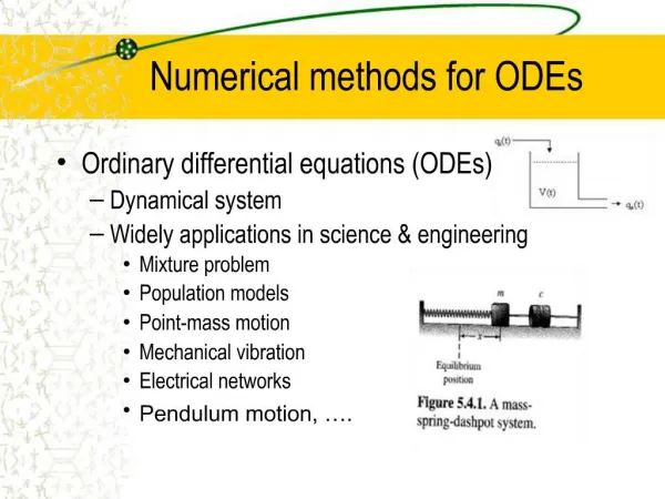
280 likes | 964 Vues
Review of numerical methods for ODEs Numerical Methods for PDEs Spring 2007. Jim E. Jones. References: Numerical Analysis, Burden & Faires Scientific Computing: An Introductory Survey, Heath. Ordinary Differential Equation: Initial Value Problem (IVP).

Review of numerical methods for ODEs Numerical Methods for PDEs Spring 2007
E N D
Presentation Transcript
Review of numerical methods for ODEs Numerical Methods for PDEs Spring 2007 Jim E. Jones • References: • Numerical Analysis, Burden & Faires • Scientific Computing: An Introductory Survey, Heath
Ordinary Differential Equation: Initial Value Problem (IVP) • Numerical Solution: rather than finding an analytic solution for y(t), we look for an approximate discrete solution wi (i=0,1,…,n) with wi approximating y(a+ih) t t=b t=a h
Forward Euler via Taylor’s Theorem Write down a Taylor expansion for y about ti Evaluate at ti+1 and note y’=f Drop h2 term to get Euler’s method (forward Euler)
Backward Euler via Taylor’s Theorem Write down a Taylor expansion for y about ti+1 Evaluate at ti and note y’=f Drop h2 term to get Euler’s method (backward Euler)
Explicit vs. Implicit Methods Forward Euler Backward Euler • Forward Euler is an explicit method. Computing the new approximation wi+1 is simple. • Backward Euler is an implicit method. Computing the new approximation wi+1 can be more complicated; it appears on both sides of the equation and inside the f function.
Ordinary Differential Equation: Example 1 Forward Euler with h=0.1 Backward Euler with h=0.1 Solving for w1 using Newton’s Method More examples at http://www.cse.uiuc.edu/iem/ode/
Ordinary Differential Equation: Example 2.a Forward Euler with h=0.1 Backward Euler with h=0.1 Both computed solutions go to zero as t increases like the true ODE solution
Ordinary Differential Equation: Example 2.b Forward Euler with h=1.1 Backward Euler with h=1.1 Backward Euler go to zero as t increases. Forward Euler blows up.
Ordinary Differential Equation: Example 2.b Forward Euler with h=1.1 We say that forward Euler is unstable. Stability is an important property of numerical methods for ODEs and PDEs. Our goal over the next few lectures will be to explain and quantify this behavior. Backward Euler with h=1.1 Backward Euler go to zero as t increases. Forward Euler blows up.
Ordinary Differential Equation: Example 2.b Forward Euler with h=1.1 To do this investigation, we will need some results from the theory of ODEs. These results are from Burden & Faires. Backward Euler with h=1.1 Backward Euler go to zero as t increases. Forward Euler blows up.
Lipschitz condition definition A function f(t,y) satisfies a Lipschitz condition in the variable y on a set D in R2 if a constant L > 0 exists with whenever (t,y0) and (t,y1) are in D. The constant L is called a Lipschitz constant for f.
Convex set definition A set D in R2 is said to be convex if whenever (t0,y0) and (t1,y1) belong to D and l is in [0,1], the point ((1-l)t0+lt1, (1-l)y0+ly1) also belongs to D. convex not convex
Theorem: bounded partial derivative a Lipschitz Suppose f(t,y) is defined on a convex set D in R2. If L is a bound on fy, i.e. then f satisfies a Lipschitz condition on D in the variable y with Lipschitz constant L.
Theorem: Lipschitz a Existence and Uniqueness Suppose that and that f(t,y) is continuous on D and satisfies a Lipschitz condition on D in the variable y, then the IVP has a unique solution y(t) for t in [a,b].
Well posed IVP definition The IVP is a well-posed problem if: • A unique solution y(t) exists, and • There exists constants e0 >0 and K > 0 such that for any e in (0,e0), whenever d(t) is continuous with |d(t)| < e for all t in [a,b], and when |d0| < e, the IVP has a unique solution z(t) satisfying
Well posed IVP definition The IVP is a well-posed problem if: • A unique solution y(t) exists, and • There exists constants e0 >0 and K > 0 such that for any e in (0,e0), whenever d(t) is continuous with |d(t)| < e for all t in [a,b], and when |d0| < e, the IVP has a unique solution z(t) satisfying Original IVP Perturbed IVP Difference in solutions to 2 IVPs
Characteristics of well-posed problems • In words, an IVP is well-posed if small perturbations in the data (the right-hand side and initial condition) produce correspondingly small changes in the solution. • When solving an IVP numerically, we can not expect reasonable results for problems that are not well-posed (Why?). Such problems are called ill-posed.
Characteristics of well-posed problems Numerical solution will always be dealing with perturbed problems due to round-off error in computer representation. If these small errors produce large changes in the solution, we can’t expect good agreement between the computed solution and the solution to the IVP • In words, an IVP is well-posed if small perturbations in the data (the right-hand side and initial condition) produce correspondingly small changes in the solution. • When solving an IVP numerically, we can not expect reasonable results for problems that are not well-posed (Why?). Such problems are called ill-posed.
Theorem: Lipschitz a Well-posed Suppose that and that f(t,y) is continuous on D and satisfies a Lipschitz condition on D in the variable y, then the IVP is well-posed.
Is the Example 2.b well-posed? Recall the Lipschitz condition or The rhs f(t,y)=-2y clearly satisfies the Lipschitz condition with L=2. So the IVP is well-posed. The blow-up of forward Euler is due to the numerical method for this IVP, not the IVP itself.
Is the Example 2.b well-posed? To investigate the problem were seeing with forward Euler, we will need to define some properties for numerical methods; namely, consistency, stability, and accuracy (or convergence). Again Burden & Faires or Heath are good references. Recall the Lipschitz condition or The rhs f(t,y)=-2y clearly satisfies the Lipschitz condition with L=2. So the IVP is well-posed. The blow-up of forward Euler is due to the numerical method for this IVP, not the IVP itself.
Local truncation error definition The difference method has local truncation error for each i=0,1,…,n-1
Local truncation error definition The difference method has local truncation error for each i=0,1,…,n-1 The local truncation error is a measure of the degree to which the true IVP solution fails to satisfy the difference equation.
Local truncation error definition The difference method has local truncation error for each i=0,1,…,n-1 The local truncation error is error in single step, assuming the previous step is exact, scaled by the mesh size h.
Local truncation error for Euler From the Taylor theorem derivation for forward Euler we had so so if y’’ is bounded, the local truncation error is O(h). Same result holds for backward Euler.
Definition of consistency and convergence A difference method is consistent with the differential equation if A difference method is convergent (or accurate) with respect to the differential equation if
Definition of consistency and convergence A difference method is consistent with the differential equation if A difference method is convergent (or accurate) with respect to the differential equation if The missing piece of the puzzle is the concept of stability of a numerical method. Next time we’ll define stability and see that Consistency + Stability = Accuracy