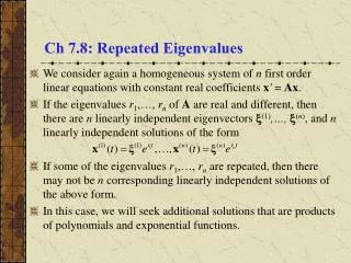
Ch 7.8: Repeated Eigenvalues
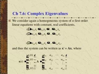
Ch 7.8: Repeated Eigenvalues. We consider again a homogeneous system of n first order linear equations with constant real coefficients x ' = Ax .

Ch 7.8: Repeated Eigenvalues
E N D
Presentation Transcript
Ch 7.8: Repeated Eigenvalues • We consider again a homogeneous system of n first order linear equations with constant real coefficients x' = Ax. • If the eigenvalues r1,…, rnof Aare real and different, then there are n linearly independent eigenvectors (1),…, (n), and nlinearly independent solutions of the form • If some of the eigenvalues r1,…, rn are repeated, then there may not be n corresponding linearly independent solutions of the above form. • In this case, we will seek additional solutions that are products of polynomials and exponential functions.
Example 1: Direction Field (1 of 12) • Consider the homogeneous equation x' = Ax below. • A direction field for this system is given below. • Substituting x = ert in for x, and rewriting system as (A-rI) = 0, we obtain
Example 1: Eigenvalues (2 of 12) • Solutions have the form x = ert, where r and satisfy • To determine r, solve det(A-rI) = 0: • Thus r1= 2 and r2= 2.
Example 1: Eigenvectors (3 of 12) • To find the eigenvectors, we solve by row reducing the augmented matrix: • Thus there is only one eigenvector for the repeated eigenvalue r = 2.
Example 1: First Solution; andSecond Solution, First Attempt (4 of 12) • The corresponding solution x = ert of x' = Ax is • Since there is no second solution of the form x = ert, we need to try a different form. Based on methods for second order linear equations in Ch 3.5, we first try x = te2t. • Substituting x = te2t into x' = Ax, we obtain or
Example 1: Second Solution, Second Attempt (5 of 12) • From the previous slide, we have • In order for this equation to be satisfied for all t, it is necessary for the coefficients of te2t and e2t to both be zero. • From the e2t term, we see that = 0, and hence there is no nonzero solution of the form x = te2t. • Since te2t and e2t appear in the above equation, we next consider a solution of the form
Example 1: Second Solution and its Defining Matrix Equations (6 of 12) • Substituting x = te2t + e2t into x' = Ax, we obtain or • Equating coefficients yields A = 2 and A = + 2, or • The first equation is satisfied if is an eigenvector of A corresponding to the eigenvalue r = 2. Thus
Example 1: Solving for Second Solution(7 of 12) • Recall that • Thus to solve (A – 2I) = for , we row reduce the corresponding augmented matrix:
Example 1: Second Solution (8 of 12) • Our second solution x = te2t + e2t is now • Recalling that the first solution was we see that our second solution is simply since the last term of third term of x is a multiple of x(1).
Example 1: General Solution (9 of 12) • The two solutions of x'= Ax are • The Wronskian of these two solutions is • Thus x(1)and x(2)are fundamental solutions, and the general solution of x' = Ax is
Example 1: Phase Plane (10 of 12) • The general solution is • Thus x is unbounded as t , and x 0as t -. • Further, it can be shown that as t -, x 0asymptotic to the line x2 = -x1 determined by the first eigenvector. • Similarly, as t , x is asymptotic to a line parallel to x2 = -x1.
Example 1: Phase Plane (11 of 12) • The origin is an improper node, and is unstable. See graph. • The pattern of trajectories is typical for two repeated eigenvalues with only one eigenvector. • If the eigenvalues are negative, then the trajectories are similar but are traversed in the inward direction. In this case the origin is an asymptotically stable improper node.
Example 1: Time Plots for General Solution (12 of 12) • Time plots for x1(t) are given below, where we note that the general solution x can be written as follows.
General Case for Double Eigenvalues • Suppose the system x' = Ax has a double eigenvalue r = and a single corresponding eigenvector . • The first solution is x(1) = e t, where satisfies (A-I) = 0. • As in Example 1, the second solution has the form where is as above and satisfies (A-I) = . • Since is an eigenvalue, det(A-I) = 0, and (A-I) = b does not have a solution for all b. However, it can be shown that (A-I) = always has a solution. • The vector is called a generalized eigenvector.
Example 2: Fundamental Matrix (1 of 2) • Recall that a fundamental matrix (t) for x' = Ax has linearly independent solution for its columns. • In Example 1, our system x'= Ax was and the two solutions we found were • Thus the corresponding fundamental matrix is
Example 2: Fundamental Matrix (2 of 2) • The fundamental matrix (t) that satisfies (0)= I can be found using (t) = (t)-1(0), where where -1(0) is found as follows: • Thus
Jordan Forms • If A is n x n with n linearly independent eigenvectors, then A can be diagonalized using a similarity transform T-1AT = D. The transform matrix T consisted of eigenvectors of A, and the diagonal entries of D consisted of the eigenvalues of A. • In the case of repeated eigenvalues and fewer than n linearly independent eigenvectors, A can be transformed into a nearly diagonal matrix J, called the Jordan form of A, with T-1AT = J.
Example 3: Transform Matrix(1 of 2) • In Example 1, our system x' = Ax was with eigenvalues r1= 2 and r2= 2 and eigenvectors • Choosing k = 0, the transform matrix T formed from the two eigenvectors and is
Example 3: Jordan Form(2 of 2) • The Jordan form J of A is defined by T-1AT = J. • Now and hence • Note that the eigenvalues of A, r1= 2 and r2= 2, are on the main diagonal of J, and that there is a 1 directly above the second eigenvalue. This pattern is typical of Jordan forms.