Download

1 / 32
320 likes | 1.65k Vues
Dispersion Modeling 101: ISCST3 vs. AERMOD. Iowa Chapter AWMA February 14, 2006 Mick Durham Stanley Consultants, Inc . What we are going to talk about. Brief History of Dispersion Modeling Industrial Source Complex Model AMS/EPA Regulatory Model (AERMOD) Comparisons The IDNR Connection

E N D
Dispersion Modeling 101:ISCST3 vs. AERMOD Iowa Chapter AWMA February 14, 2006 Mick Durham Stanley Consultants, Inc.
What we are going to talk about • Brief History of Dispersion Modeling • Industrial Source Complex Model • AMS/EPA Regulatory Model (AERMOD) • Comparisons • The IDNR Connection • Questions & Answers
Brief History of Modeling • Earliest Studies Simulated the Movement of Air • G.I. Taylor, 1915, Eddy Motion in the Atmosphere • O.G. Sutton, 1932, A Theory of Eddy Diffusion • Dispersion of Pollutants (Mainly Particulate) Followed WW II • E.W. Hewson, 1945, Meteorological Control of Atmospheric Pollutants by Heavy Industry • E.W. Hewson, 1955, Stack Heights Required to Minimize Ground Level Concentrations • Gale, Stewart & Crooks, 1958, The Atmospheric Diffusion of Gases Discharged from a Chimney
Brief History of Modeling • Birth of Dispersion Parameters • F.A. Gifford, 1960, Atmospheric Dispersion Calculations Using the Gaussian Plume Model • F. Pasquill, 1961, The Estimation of the Dispersion of Windborne Material • D. Bruce Turner, 1967, Workbook on Atmospheric Dispersion Estimates • Briggs, Gary, 1969, Plume Rise
Brief History of Modeling • Modeling and the Computer Age • PTMAX, PTMIN, PTMTP, 1972 • Air Quality Display Model (AQDM), 1974 • Single Source (CRSTER) Model, 1977 • Complex Terrain (VALLEY) Model, 1977 • Multiple Source (MPTER) Model, 1980 • Pollutant and Environment Specific Models • APRAC, CALINE, HIWAY Carbon Monoxide Models • BLP (Bouyant Line and Point Sources); PAL (Point Area and Line Source), 1979; TEM (Texas Episode for Urban Areas) • RPM (Reactive Plume Model) for Ozone, 1980
Brief History of Modeling • Guideline on Air Quality Models • The Guidelines on Air Quality Models, 1978 • 40 CFR Part 58, Appendix W • Refined and More Complex Models • Industrial Source Complex (ISC), 1979 • Industrial Short-Term ST • Industrial Long-Term LT • Complex Terrain (COMPLEX) • Dense Gas (DEGADIS) • Urban Airshed Model (UAM)
Brief History of Modeling • Refined and More Complex Models (cont.) • Screening Model (SCREEN) • California Line Source (CALINE) and Mobile Source Emission Factors (MOBILE) • Puff Models (INPUFF) • Visibility (VISCREEN)
Brief History of Modeling • Advanced Models • Industrial Source Complex Version 2 (ISC2), 1990 • Industrial Source Complex Version 3 (ISC3), 1995 • California Line Source (CAL3QH3) • Urban Airshed Model (UAM-V) • Complex Terrain Dispersion Model (CTDMPLUS) • Offshore and Coastal Dispersion Model (OCD) • Bouyant Line and Point Source (BLP) • Area Locations of Hazardous Atmospheres (ALOHA) • Dense Gas Dispersion Model (DEGADIS 2.1)
Brief History of Modeling • Today’s Models: • AERMOD • Point, Area, Line Sources • Simple or Complex Terrain • Transport distance up to 50 km • CALPUFF • Transport from 50 to hundreds of kilometers • Visibility, Regional Haze • Dispersion in Complex Terrain • Complex Dispersion Model Plus Algorithms for Unstable Conditions (CTDMPLUSS) • Dispersion in Complex Terrain
Brief History of Modeling • Today’s Models (Continued): • Caline3 or CAL3QHC, MOBILE6 • Highway Line sources • Simple Terrain • Carbon Monoxide • Buoyant Line and Point Source (BLP) • Aluminum Reduction plants with buoyant line and point sources • Rural location • Simple Terrain • Community Multi-scale Air Quality Model (CMAQ) • Ozone
Industrial Source Complex Model • Introduced in 1979 • First adopted as Preferred Model in 1983 • Major Revisions 4 times in 27 year history • Can remain acceptable as a preferred model until November 9, 2006
Industrial Source Complex Model • Gaussian Plume Model • Building Downwash • Particulate Deposition • Point, Area, and Line Sources • Complex Terrain • Simple Meteorological Data Input
Industrial Source Complex Model • Has been primary model in Iowa for 27 years • Over 100 facilities have modeled compliance with ISC • Generally the short-term standards have caused greatest predicted non-compliance
Industrial Source Complex Model • Problems with ISCST3: • Modeling of Plume Dispersion is Crude • Only 6 possible states (Stability Classes) • No variation in most meteorological variables with height • No use of observed turbulence data • No information about surface characteristics • Erroneous depiction of dispersion in convective conditions • Substantial overprediction in complex terrain • Crude building downwash algorithm
AERMOD • AERMOD stands for American Meteorological Society/ Environmental Protection Agency Regulatory Model • Formally Proposed as replacement for ISC in 2000 • Adopted as Preferred Model November 9, 2005
AERMOD • 3 COMPONENTS • AERMET – THE METEOROLOGICAL PREPROCESOR • AERMAP – THE TERRAIN DATA PREPROCESSOR • AERMOD – THE DISPERSION MODEL • 2 SUPPORT TOOLS • AERSURFACE – PROCESSES SURFACE CHARACTERISTICS DATA • AERSCREEN – PROVIDES A SCREENING TOOL
AERMOD • AERMOD IS SIMILAR TO ISC IN SETUP • THE CONTROL FILE STRUCTURE IS THE SAME • VIRTUALLY ALL THE CONTROL KEYWORDS AND OPTIONS ARE THE SAME
AERMOD • AERMOD IS DIFFERENT FROM ISC • REQUIRES SURFACE CHARACTERISTICS (ALBEDO, BOWEN RATIO, SURFACE ROUGHNESS) IN AERMET • HAS PRIME FOR BUILDING DOWNWASH AND THE BUILDING PARAMETERS ARE MORE EXTENSIVE • REQUIRES LONGER COMPUTER RUN TIMES (up to 5 times longer!)
Comparison of Dispersion Model Features:Meteorological Data Input • – ISCST3: • One level of data accepted • – AERMOD: • An arbitrarily large number of data levels can be accommodated
Comparison of Dispersion Model Features:Plume Dispersion and Plume Growth Rates ISCST3: • Based upon six discrete stability classes only • Dispersion curves are Pasquill-Gifford • Choice of rural or urban surfaces only AERMOD: • Uses profiles of vertical and horizontal turbulence variable with height • Uses continuous growth function • Uses many variations of surface characteristics
Comparison of Dispersion Model Features:Complex Terrain Modeling ISCST3: • Elevation of each receptor point input • Predictions are very conservative in complex terrain AERMOD: • Controlling hill elevation and point elevation at each receptor are input • Predictions are nearly unbiased in complex terrain
Comparisons ISC Vs AERMOD CONSEQUENCE ANALYSIS - ratios of AERMOD predicted high concentrations to ISCST3 predicted high concentrations: flat and simple terrain point, volume and area sources. 1hour 3hour 24hour annual average 1.04 1.09 1.14 1.33 high 4.25 2.82 3.15 3.89 low 0.32 0.26 0.24 0.30 Total 48 48 48 48 • AN OVERVIEW FOR THE 8TH MODELING CONFERENCE SEPTEMBER 22, 2005
Comparisons ISC Vs AERMOD CONSEQUENCE ANALYSIS - ratios of AERMOD predicted high concentrations to ISCST3 (and PRIME) predicted high concentrations: flat terrain point sources with significant bldg downwash ANNUAL 24 H2H3 H2H AER/ISC3AER/ISCPAER/ISC3AER/ISCPAER/ISC3AER/ISCP ave 1.08 1.05 1.25 1.01 0.71 1.05 max 1.35 1.29 1.87 1.14 1.20 1.17 min 0.69 0.79 0.69 0.84 0.38 0.93 No cases 6 6 6 • AN OVERVIEW FOR THE 8TH MODELING CONFERENCE SEPTEMBER 22, 2005
Comparisons ISC Vs AERMOD • Duane Arnold Energy Center Data (Palo, IA) • Ratio of Modeled Conc to Observed: • AERMOD: 0.69 (1-hr avg 46m release) • ISC-Prime: 0.76 (1-hr avg 46m release) • AERMOD: 0.25 (1-hr avg 24m release) • ISC-Prime: 0.29 (1-hr avg 24m release) • AERMOD: 0.51 (1-hr avg 1m release) • ISC-Prime: 0.38 (1-hr avg 1m release)
Comparisons ISC Vs AERMOD • Presentation at EUEC conference by Bob Paine, TRC: • AERMOD consistently showed better or comparable performance with ISCST3 • In flat terrain, AERMOD and ISCST3 predictions are comparable, but AERMOD has higher annual averages • In complex terrain, AERMOD predictions are markedly lower • Building downwash predictions will often be lower, especially for stacks located some distance from controlling buildings • Overall, more confidence in accuracy of AERMOD results
Comparisons ISC Vs AERMOD • Our Recent Experience: • Annual concentrations higher with AERMOD by 10-15% • Short term concentrations similar without downwash • Short-term concentrations generally lower with building downwash by 20%
The IDNR Connection • IDNR will allow use of either ISCST3 or AERMOD until November 9, 2006 • Meteorological Data will be provided by IDNR for eight stations • Compliance with ISCST3 and non-compliance by AERMOD must be addressed