Download
1 / 25
250 likes | 268 Vues
This paper examines the concepts of self-configuration and self-healing in wireless networks, with a focus on scalability and locality. It explores the use of geographic information to optimize communication quality, energy dissipation, and data aggregation. The paper also discusses strategies for static and dynamic networks, including intra-cell and inter-cell healing mechanisms.

E N D
GS3: Scalable Self-configuration and Self-healing in Wireless Networks Hongwei Zhang & Anish Arora
Introduction • Sensor networks are not deployed manually self-configuration (into interconnected clusters) • Sensor nodes and wireless links are subject to a rich class of faults self-healing (of clusters and interconnections) • Sensor networks need to scale well in time, space, and resources scalability in self-configuration and self-healing
Scalability via locality • An ideal goal for locality : self-healing should be a function of the size of perturbation (in time, space, and energy) • Example: problem of dining philosophers • for correctness: dining philosophers need “information” only from philosophers at distance ≤ 2 hops • for fault-tolerance: (Nesterenko and Arora’02) • if state corruptions occur within a 2-hop neighborhood, they can be corrected within the neighborhood itself • any number of Byzantine philosophers can be tolerated as long as they are ≥ 2 hops away
Locality via choice of model • Locality for some graph problems is hard • e.g. self-configuration and self-healing of routing tree • Our approach to simplifying design of locality • choose a proper model for specific problems
System model • System • multiple “small” nodes and one “big” node, on a plane • node distribution • density: ( Rts.t. with high probability, there are multiple nodes in any circular area of radius Rt) • localization: relative location between nodes can be estimated • Perturbations • dynamic nodes • joins, leaves (deaths), state corruptions • mobile nodes
Geography-aware self-configuration • Geographic radius of clusters is crucial • for communication quality, energy dissipation, data aggregations & applications • Problem statement • Given R: ideal cell radius (R > Rt) • Construct a set of cells , connected via a “head” node in each cell s.t. • radius of each cell is in [ R-c , R+c ] , where c = f (Rt) • each node belongs to only one cell • cells and the connectivity graph over head nodes self-heal locally
Outline • Static networks • Dynamic networks • Mobile dynamic networks • Related work • Conclusions
Static networks • An ideal case: • In reality: no node may exist at some geometric centers (ILs), but, with high probability there are nodes no more than Rt away from any IL (IL = Ideal Location)
How to find the set of cell heads • Bottom-up ? • hard to guarantee the placement and size of clusters • Top-down w.r.t. big node • use diffusing computation • but, accumulation in deviation of head location from IL is a problem i
Organizing neighboring clusters & heads Deviation problem is handled locally • instead of using real locations, node i uses its and its parent’s ILs • i calculates the ILs of next band cells in its search region < LD , RD > • big node: <0o , 360o> • other nodes: <-60o-a , 60o+a> , where a Sin-1(Rt / R) • for each IL, i ranks nodes within Rt radius of the IL (by <D, A>), and selects the highest ranked node as the corresponding cluster head
Summary: static networks • Cell structure is hexagonal • cell radius: • Time taken to form the structure is (Db), where Db = the maximum distance between the big node and the small nodes • Scalability in self-configuration: • local coordination: only with nodes within range • local knowledge: each node maintains info about a constant number of nearby nodes
Outline • Static networks • Dynamic networks • Mobile dynamic networks • Related work • Conclusions
Dynamic networks • Dynamics include: • node join, leave (death), state corruption • Common vs. rare • common perturbations: node density is preserved • rare perturbations: node density is destroyed • Scalable self-healing is achieved via locality in: • intra-cell healing • inter-cell healing • sanity checking of state (invariants)
Local intra-cell healing • Head shift • upon head leaving (death) • local in a radius of Rt • Cell shift • upon the death of all the nodes in an area of radius Rt • local in a radius of R • independent but consistent shift at individual cells sliding of the global head level structure
H0 H0 H0 H0
Local inter-cell healing & sanity checking • Local inter-cell healing : upon failure of intra-cell healing at head j, • first, the parent of j tries to find a new head j’ • if that fails, the children of j find new parents • Local sanity checking of state invariants : upon detecting violation of the hexagonality property, • node corrects itself after checking with its neighbors • when state perturbation includes several nodes, the perturbed region corrects itself from the outside going in, and all nodes are corrected within time proportional to size of perturbed region
Summary: dynamic networks • Cell radius • for cells not adjoining any gap: • for cells adjoining a gap: • Head tree is now minimum distance tree rooted at the big node • Stabilization time from perturbed state: (Dp), where Dp = diameter of the continuously perturbed area
Summary: dynamic networks (contd.) • Scalability in self-healing: • local fault-containment and healing • local knowledge • Local healing and fault-containment enables • stable cell structure • lengthened lifetime: (nc) , where nc = the number of nodes in a cell
Outline • Static networks • Dynamic networks • Mobile dynamic networks • Related work • Conclusions
Mobile dynamic networks H0 d H0
Outline • Static networks • Dynamic networks • Mobile dynamic networks • Related work • Conclusions
Related work • Cellular hexagon structure (Mac Donald ’79) • Preconfigured & not considering self-healing • LEACH (Heinzelman et al’00) • No guarantee about the placement and size of clusters • Perturbations dealt with by globally repeating the whole clustering process
Related work (contd.) • Logical-radius based clustering (in Banerjee ’01) • non-local cluster maintenance, and no consideration of state corruption • only logical radius long links and link asymmetry are possible • multiple rounds of diffusion • Self-stabilization • tree maintenance (in Arora & Gouda ’90) • not fault containing • local mending (in Kutten & Peleg ’95) • local in time, not in space
Outline • Static networks • Dynamic networks • Mobile dynamic networks • Related work • Conclusions
Conclusions • GS3 is scalable • self-configuration • self-healing • And this is achieved by exploiting the model properties in wireless sensor networks • Density • Localization (Note: we have also designed an algorithm for “local containment of faults in general spanning trees” for dynamic networks)