Space Shuttle limb view
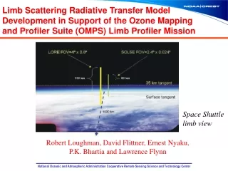
Limb Scattering Radiative Transfer Model Development in Support of the Ozone Mapping and Profiler Suite (OMPS) Limb Profiler Mission. Space Shuttle limb view. Robert Loughman, David Flittner, Ernest Nyaku, P.K. Bhartia and Lawrence Flynn. SOLAR IRRADIANCE. MULTIPLE SCATTERING. SATELLITE.


Space Shuttle limb view
E N D
Presentation Transcript
Limb Scattering Radiative Transfer Model Development in Support of the Ozone Mapping and Profiler Suite (OMPS) Limb Profiler Mission Space Shuttle limb view Robert Loughman, David Flittner, Ernest Nyaku, P.K. Bhartia and Lawrence Flynn
SOLAR IRRADIANCE MULTIPLE SCATTERING SATELLITE LINE OF SIGHT SINGLE SCATTERING TANGENT HEIGHT CLOUDS SURFACE Outline • Review of OMPS and Limb Scattering (LS) • Reasons for studying stratospheric aerosol • Improving the OMPS LS Radiative Transfer Model • Conclusions and Future Work
OMPS Mission • OMPS launched on the Suomi NPP satellite in October 2011 • The mission of OMPS is to continue the long-term ozone record for trend assessment • But the properties of other species (such as aerosol) must also be known to achieve the desired ozone retrieval performance OMPS = Ozone Mapping and Profiler Suite LP = Limb Profiler
Why worry about Stratospheric Aerosol? • Poor estimates of stratospheric aerosol → poor ozone profile retrievals. • Stratospheric aerosol has a significant cooling effect on climate: Some radiation that would have reached the lower atmosphere is instead reflected back to space. • Important questions persist about the processes that govern stratospheric aerosol:
Why worry about Stratospheric Aerosol? • Solomon et al. (2011) challenges the simplistic model that the stratosphere has a well-defined “background aerosol level” that is perturbed by irregular volcanic eruptions (such as Pinatubo). • Brief summary: Recent measurements show that stratospheric aerosol is changing in unexpected ways (~50% increase from its minimum level, despite a notable lack of explosive volcanic eruptions). • Bottom line: Failure to capture these stratospheric aerosol changes may lead climate models to make poor predictions of future temperature variations.
Why worry about Stratospheric Aerosol? • Bourassa et al. (2012), Fromm et al. (2013), Vernier et al. (2013) and finally Bourassa et al. (2013) have engaged in a spirited debate concerning recent measurements of stratospheric aerosol. • Brief summary: All agree that the 2011 Nabro eruption caused aerosol to appear in the stratosphere, but they sharply disagree about how it got there – injection, or transport, or both? • Bottom line: Debates about the mechanisms that control the abundance of aerosol in the stratosphere continue. Recent analyses have shown that tropospheric aerosol can be injected into the stratosphere (e.g., during forest fires, Fromm et al., 2010). If tropospheric injection is a significant source of stratospheric aerosol, that has significant implications for future climate.
OMPS LP Radiative Transfer • The OMPS ozone and aerosol profile retrieval algorithms fundamentally depend upon comparing measured radiances to calculated radiances. • The level of agreement between these two sets of radiances is a key part of our assessment of the OMPS instrument. • The calculated radiances in the OMPS come from a version of the GSLS radiative transfer model (RTM) that has been highly optimized for speed. • In the past year, I was asked by the OMPS Science Team to revisit the RTM, with the aim of repairing some known defects that cause systematic errors in the calculated radiances.
Single-scattering comparison to Siro benchmark • Wavelengths are 325, 345, and 600 nm • Azimuth angles = 20° (solid), 90° (dashed), and 160°(dot-dashed) • Solar zenith angles (SZA) = 15° & 60° (left), 80° & 90° (right) • Thin line = smaller SZA, thick line = larger SZA in each picture
Refinement of atmospheric representation • A known deficiency (see Loughman et al., 2004) of the GSLS model concerns its calculation of the optical path length τ through an atmospheric layer, given the extinction coefficient β and path length s: • GSLS model (for all but the tangent layer) makes an error that → 1% as θ → 90°: τ= s * (layer avgβ) • Updated model: τ= ∫ β ds • (allowing β to vary as a linear function of height) • (NOTE that the Siro benchmark model uses the updated model’s approach)
GSLS RTM approximate MS Multiple scattering is calculated at just one zenith: ↓ • This approximation minimizes the time required for multiple scattering MS - the slowest step in the RTM calculation • But it leads to large radiance errors for cases when the radiation field varies rapidly along the line of sight Fig. 9 of Loughman et al. (2004)
Updated RTM MS can be calculated at several zeniths: ↓ ↓ ↓ ↓ ↓ • This model is several times slower than GSLS, but it allows us to better simulate: • Broken cloud fields • Horizontal variation of atmospheric properties • Near-twilight conditions Fig. 9 of Loughman et al. (2004)
Multi-zenith MS improvement • Same wavelengths and azimuth angles as previously • Concentrate on total radiance for large SZA (> 80°) cases • Left panel: GSLS calculations, 1 MS zenith • Right panel: Current calculations, 17 MS zeniths
GSLS scalar radiance error • The GSLS model used for OMPS LP retrievals also neglects polarization, and instead calculates approximate (scalar) radiances. • This approximation decreases the RTM computational burden, and has little influence on the retrieval algorithms, but it produces significant radiance errors (up to 12% worst case) • The updated model has restored the capability to make correct (vector) radiance calculations • The scalar radiance error is shown on the following slides for a simulated OMPS LP orbit
OMPS Variation of single-scattering angle • Small event number: Early orbit, Southern Hem., large scat. angle, back-scatter view • Large event number: Late orbit, Northern Hem., small scat. angle, forward-scat. view
Scalar radiance error at 40 km Error is shown for λ = 325, 345, 385, 400, 449,521 nm (solid lines) and 602, 676, 756, 869, 1020 nm (dashed line) Same scalar radiance error pattern prevails for all wavelengths Amplitude approaches 10 % at 345 nm (-3.5% to +5.5%), for R = 0.3
Stratospheric ASD measurements • At z = 20 km the aerosol size distribution (ASD) tends to contain larger particles, relative to z = 25 km • Recent RTM updates allow us to simulate this variation Thanks to Deshler et al. for balloon measurements of aerosol properties at Laramie, Wyoming, 2012
ASD effect on radiance, 676 nm The radiance difference is shown for TH = 20, 25, 30, 35, 40 km The ASD effect exceeds ±20% for a broad portion of the orbit
Conclusionsand Future Work • OMPS LP instrument and retrieval algorithms are performing well • But the more accurate RTM described herein will help us understand the measurements better, and enable retrievals for previously unpromising situations (large SZA, broken cloud fields, variable aerosol properties, etc.) • Systematically analyze the impact of these RTM improvements in the ozone and aerosol retrievals • Develop innovative retrievals that extract more useful information from OMPS LP radiance data.
Acknowledgements • NASA NPP Science Team and NOAA / CREST for supporting LS research • Didier Rault, for his work leading the development of the OMPS LP retrieval algorithm • The OSIRIS, SCIAMACHY, SAGE II, SAGE III, and U. of Wyoming measurement teams, for maintaining and sharing their high-quality data sets • Ghassan Taha, Zhong Chen, Nick Gorkavyi, Philippe Xu, and Leslie Moy for helpful discussions • Daryl Ludy, Ricardo Uribe and Curtis Driver for their help with testing the algorithms as students
Updated Model (Review) MS can be calculated at several zeniths: ↓ ↓ ↓ ↓ ↓ • So far, I’ve: • Stripped down LP_RAD_SIMUL to make a single-wavelength, single-zenith model. • Verified that the single-wavelength, single-zenith model replicates the Loughman et al. (2004) calculations for Rayleigh and Rayleigh + HG aerosol cases (in both scalar and vector modes). • Begun to experiment with MS calculations at multiple zeniths. Fig. 9 of Loughman et al. (2004)
Refinement of atmospheric representation • A known deficiency of the GSLS and LP_RAD_SIMUL models concerns its calculation of the optical path length τ through an atmospheric layer (path length = s): • Current model: τ = s * (layer avg ext coef) • Updated model: τ = ∫ (ext coef) ds • (allowing ext coef to vary as a linear function of height) • NOTE: Siro (benchmark) model uses the updated approach
SS comparison to Siro • Wavelengths are 325, 345, and 600 nm • Azimuth angles = 20 (solid), 90 (dashed), and 160 (dot- dashed) deg • Solar zenith angles are 15, 60, 80 and 90 deg • Thin line = smaller SZA, thicker line = larger SZA in each picture • Top panel: L04 calculations (constant ext coef within each layer) • Bottom panels: Current calculations (ext coef is a linear f(height) within each layer)
Now add multiple zeniths • Same wavelengths (325, 345, and 600 nm) • Same azimuth angles (20, 90 and 160 deg) • Same solar zenith angles, except that 90 deg is excluded (model fails for MS calculation below horizon), so only (15, 60 and 80 deg) remain • Top panel: Current calculations, 1 MS zenith • Bottom panel: Current calculations, 17 MS zeniths
Aerosol Jacobians for event 151 (SSA = 24°) Surface reflectivity = 0 λ = 325 nm
Aerosol Jacobians for event 151 (SSA = 24°) Surface reflectivity = 0 λ = 385 nm
Aerosol Jacobians for event 151 (SSA = 24°) Surface reflectivity = 0 λ = 521 nm
Aerosol Jacobians for event 151 (SSA = 24°) Surface reflectivity = 0 λ = 756 nm
Aerosol Jacobians for event 151 (SSA = 24°) Surface reflectivity = 0 λ = 1020 nm
ASD measurements • To see how these ASDs affect the extinction coefficient and phase function, I made calculations using the average characteristics for z = 20 km and z = 25 km (averaging over the 6 Laramie measurements from 2012):
ASD measurements • At z = 20 km the distribution contains larger particles, relative to z = 25 km Thanks to Deshler et al., balloon measurements at Laramie, Wyoming, 2012
OMPS Variation of single-scattering angle • Small event number: Early orbit, Southern Hem., large scat. angle, back-scatter view • Large event number: Late orbit, Northern Hem., small scat. angle, forward-scat. view
Difference in phase function, 449 nm Total phase function shown for TH = 20, 25, 30, 35, 40 km Solid = ASD20, dashed = ASD25 Black line = Rayleigh As Rayleigh scattering weakens, the aerosol difference has a larger effect on the overall phase function, over a broader range of events
Change in radiance, 676 nm Difference shown for TH = 20, 25, 30, 35, 40 km Effect covers a broad portion of the orbit, and exceeds ±20%
Scalar radiance error at 40 km Error is shown for λ = 325, 345, 385, 400, 449,521 nm (solid lines) and 602, 676, 756, 869, 1020 nm (dashed line) Same scalar radiance error pattern prevails for all wavelengths Amplitude approaches 10 % at 345 nm (-3.5% to +5.5%), for R = 0.3