Download
1 / 38
390 likes | 591 Vues
390-Elliptic Curves and Elliptic Curve Cryptography. Michael Karls. Outline. Groups, Abelian Groups, and Fields Elliptic Curves Over the Real Numbers Elliptic Curve Groups Elliptic Curves Over a Finite Field An Elliptic Curve Cryptography Scheme—Diffie-Hellman Key Exchange.

E N D
390-Elliptic Curves and Elliptic Curve Cryptography Michael Karls
Outline • Groups, Abelian Groups, and Fields • Elliptic Curves Over the Real Numbers • Elliptic Curve Groups • Elliptic Curves Over a Finite Field • An Elliptic Curve Cryptography Scheme—Diffie-Hellman Key Exchange
Group Definition • A group is a non-empty set G equipped with a binary operation * that satisfies the following axioms for all a, b, c in G: • Closure: a*b in G • Associativity: (a*b)*c = a*(b*c) • Identity: There exists an element e in G such that a*e = a = e*a. We call e the identity element of G. • Inverse: For each a in G, there exists an element d in G such that a*d = e = d*a. We call d the inverse of a.
Group Definition (cont.) • If a group G also satisfies the following axiom for all a, b in G: • Commutativity: a*b = b*a, we say G is an abelian group. • The order of a group G, denoted |G| is the number of elements in G. If |G| < , we say G has finite order.
Group Examples • One example of a group is the set of real numbers with addition. • Another group can be made from the set of permutations on the set T = {1, 2, … , n}. • Recall that a permutation is a 1-1 onto function from T ! T. • When n = 3, the set of permutations on T is S3 = {(1) , (12), (13), (23), (123), (132)}. • Recall that in cycle notation, for = (12), (1) = 2, (2) = 1, and (3) = 3. • For permutations and , define the product to be the permutation obtained by applying first, then . • For example, with = (13) and = (12), = (13)(12) = (132) and = (12)(13) = (123).
Group Examples • Here is the “multiplication” table for S3: • From the table, we see that S3 is closed under this product, the identity element is (1), each element has an inverse, and the product is associative. • Therefore, S3 is a group! • We call Sn the Symmetric Group on n elements. • Which of these examples are finite? • Which are abelian?
Field Definition • A field F is a non-empty set with two binary operations, usually denoted + and *, which satisfy the following axioms for all a, b, c in F: • a+b is in F • (a+b)+c = a+(b+c) • a+b = b+a • There exists 0F in F such that a+0F = a = 0F+a. We call 0F the additive identity. • For each a in F, there exists an element x in F such that a+x = 0F = x+a. We call x the additive inverse of a and write x = -a.
Field Definition (cont.) • Field axioms (cont.): For all a, b, c in F, • a*b in F • (a*b)*c = a*(b*c) • a*b = b*a • There exists 1F in F, 1F 0F, such that for each a in F, a*1F = a = 1F*a. We call 1F the multiplicative identity. • For each a 0F in F, there exists an element y in F such that a*y = 1F = y*a. We call y the multiplicative inverse of a and write y = a-1. • a*(b+c) = a*b + a*c and (b+c)*a = b*a + c*a. (Distributive Law)
Field Examples • Note that any field is an abelian group under + and the non-zero elements of a field form an abelian group under *. • Some examples of fields: • Real numbers • Zp, the set of integers modulo p, where p is a prime number is a finite field. • For example, Z7 = {0, 1, 2, 3, 4, 5, 6} and Z23 = {0, 1, 2, 3, … , 22}.
Elliptic Curves Over the Real Numbers • Let a and b be real numbers. An elliptic curve E over the field of real numbers R is the set of points (x,y) with x and y in R that satisfy the equation together with a single element , called the point at infinity. • There are other types of elliptic curves, but we’ll only consider elliptic curves of this form. • If the cubic polynomial x3+ax+b has no repeated roots, we say the elliptic curve is non-singular. • A necessary and sufficient condition for the cubic polynomial x3+ax+b to have distinct roots is 4a3 + 27 b2 0. • In what follows, we’ll always assume the elliptic curves are non-singular.
y2 = x3-7x+6 y2 = x3-2x+4 Examples of Elliptic Curves
An Elliptic Curve Lemma • The next result provides a way to turn the set of points on a non-singular elliptic curve into an abelian group! • Elliptic Curve Lemma:Any line containing two points of a non-singular elliptic curve contains a unique third point of the curve, where • Any vertical line contains , the point at infinity. • Any tangent line contains the point of tangency twice.
Geometric Elliptic Curve Addition • Using the Elliptic Curve Lemma, we can define a way to geometrically “add” points P and Q on a non-singular elliptic curve E! • First, define the point at infinity to be the additive identity, i.e. for all P in E, P + = P = + P. • Next, define the negative of the point at infinity to be - = .
Geometric Elliptic Curve Addition (cont.) • For P = (xP,yP), define the negative of P to be -P = (xP,-yP), the reflection of P about the x-axis. • From the elliptic curve equation, we see that whenever P is in E, -P is also in E.
Geometric Elliptic Curve Addition (cont.) • In what follows, assume that neither P nor Q is the point at infinity. • For P = (xP,yP) and Q = (xQ,yQ) in E, there are three cases to consider: • P and Q are distinct points with xP xQ. • Q = -P, so xP = xQ and yP = - yQ. • Q = P, so xP = xQ and yP = yQ.
By the Elliptic Curve Lemma, the line L through P and Q will intersect the curve at one other point. Call this third point -R. Reflect the point -R about the x-axis to point R. P+Q = R y2 = x3-7x+6 Geometric Case 1: xP xQ
In this case, the line L through P and Q = -P is vertical. By the Elliptic Curve Lemma, L will also intersect the curve at . P+Q = P+(-P) = It follows that the additive inverse of P is -P. y2 = x3-2x+4 Geometric Case 2: xP = xQ and yP= - yQ
Since P = Q, the line L through P and Q is tangent to the curve at P. If yP = 0, then P = -P, so we are in Case 2, and P+P = . For yP 0, the Elliptic Curve Lemma says that L will intersect the curve at another point, -R. As in Case 1, reflect -R about the x-axis to point R. P+P = R Notation: 2P = P+P y2 = x3-7x+6 Geometric Case 3: xP=xQ and yP = yQ
Geometric Elliptic Curve Model • For an interactive illustration of how geometric elliptic addition works, a great resource is Certicom’s Geometric Elliptic Curve Model. • For the elliptic curves y2 = x3-7x+6 and y2 = x3-2x+4, try adding points P and Q or doubling P (i.e. 2 P = P+P), graphically.
Algebraic Elliptic Curve Addition • Geometric elliptic curve addition is useful for illustrating the idea of how to add points on an elliptic curve. • Using algebra, we can make this definition more rigorous! • As in the geometric definition, the point at infinity is the identity, - = , and for any point P in E, -P is the reflection of P about the x-axis.
Algebraic Elliptic Curve Addition (cont.) • In what follows, assume that neither P nor Q is the point at infinity. • As in the geometric case, for P = (xP,yP) and Q = (xQ,yQ) in E, there are three cases to consider: • P and Q are distinct points with xP xQ. • Q = -P, so xP = xQ and yP = - yQ. • Q = P, so xP = xQ and yP = yQ.
Algebraic Case 1: xP xQ • First we consider the case where P = (xP,yP) and Q = (xQ,yQ) with xP xQ. • The equation of the line L though P and Q is y = x+, where • In order to find the points of intersection of L and E, substitute x + for y in the equation for E to obtain the following: • The roots of (2) are the x-coordinates of the three points of intersection. • Expanding (2), we find:
Algebraic Case 1: xP xQ (cont.) • Since a cubic equation over the real numbers has either one or three real roots, and we know that xP and xQ are real roots, it follows that (3) must have a third real root, xR. • Writing the cubic on the left-hand side of (3) in factored form we can expand and equate coefficients of like terms to find
Algebraic Case 1: xP xQ (cont.) • We still need to find the y-coordinate of the third point, -R = (xR,-yR) on the curve E and line L. • To do this, we can use the fact that the slope of line L is determined by the points P and -R, both of which are on L: • Thus, the sum of P and Q will be the point R = (xR, yR) with where
Algebraic Case 2: xP = xQ and yP= - yQ • In this case, the line L through P and Q = -P is vertical, so L contains the point at infinity. • As in the geometric case, we define P+Q = P+(-P) = , which makes P and -P additive inverses.
Algebraic Case 3: xP=xQ and yP = yQ • Finally, we need to look at the case when Q = P. • If yP = 0, then P = -P, so we are in Case 2, and P+P = . • Therefore, we can assume that yP 0. • Since P = Q, the line L through P and Q is the line tangent to the curve at (xP,yP).
Algebraic Case 3: xP=xQ and yP = yQ • The slope of L can be found by implicitly differentiating the equation y2 = x3 + ax + b and substituting in the coordinates of P: • Arguing as in Case 1, we find that P+P = 2P = R, with R = (xR,yR), where
Elliptic Curve Groups • From these definitions of addition on an elliptic curve, it follows that: • Addition is closed on the set E. • Addition is commutative. • is the identity with respect to addition. • Every point P in E has an inverse with respect to addition, namely -P. • The associative axiom also holds, but is “hard” to prove.
Elliptic Curves Over Finite Fields • Instead of choosing the field of real numbers, we can create elliptic curves over other fields! • Let a and b be elements of Zp for p prime, p>3. An elliptic curve E over Zp is the set of points (x,y) with x and y in Zp that satisfy the equation together with a single element , called the point at infinity. • As in the real case, to get a non-singular elliptic curve, we’ll require 4a3 + 27 b2 (mod p) 0 (mod p). • Elliptic curves over Zp will consist of a finite set of points!
Addition on Elliptic Curves over Zp • Just as in the real case, we can define addition of points on an elliptic curve E over Zp, for prime p>3. • This is done in the essentially the same way as the real case, with appropriate modifications.
Addition on Elliptic Curves over Zp (cont.) • Suppose P and Q are points in E. • Define P + = + P = P for all P in E. • If Q = -P (mod p), then P+Q = . • Otherwise, P+Q = R = (xR,yR), where
Elliptic Curves Over Z23 Model • Again, Certicom provides a model for an elliptic curve over a finite field: Finite Geometric Elliptic Curve Model. • For the elliptic curves y2 = x3+16x+6 and y2 = x3+21x+4 over the field Z23, try adding points P and Q or doubling P (i.e. 2P =P+P).
Cryptography on an Elliptic Curve • Using an elliptic curve over a finite field, we can exchange information securely! • For example, we can implement a scheme invented by Whitfield Diffie and Martin Hellman in 1976 for exchanging a secret key.
Diffie-Hellman Key Exchange via Colors of Paint • Alice and Bob each have a three-gallon bucket that holds paint. • Alice and Bob choose a public color of paint, such as yellow. • Alice chooses a secret color, red. • Alice mixes one gallon of her secret color, red, with one gallon of yellow and sends the mixture to Bob. • Bob chooses a secret color, purple. • Bob mixes one gallon of his secret color, purple, with one gallon of yellow and sends the mixture to Alice.
Diffie-Hellman Key Exchange via Colors of Paint (cont.) • Alice adds one gallon of her secret color, red to the mixture from Bob. Alice ends up with a bucket of one gallon each of yellow, purple, and red paint. • Bob adds one gallon of his secret color, purple, to the mixture from Alice. Bob ends up with a bucket one gallon each of yellow, red, and purple paint. • Both Alice and Bob will have a bucket of paint with the same color—this common color is the key! • Note that even if eavesdropper Eve knows that the common color is yellow, or intercepts the paint mixtures from Alice or Bob, she will not be able to figure out Alice’s or Bob’s secret color!
Alice and Bob publicly agree on an elliptic curve E over a finite field Zp. Next Alice and Bob choose a public base point B on the elliptic curve E. Alice chooses a random integer 1<<|E|, computes P= B, and sends P to Bob. Alice keeps her choice of secret. Bob chooses a random integer 1<<|E|, computes Q = B, and sends Q to Alice. Bob keeps his choice of secret. Alice and Bob choose E to be the curve y2 = x3+x+6 over Z7. Alice and Bob choose the public base point to be B=(2,4). Alice chooses = 4, computes P = B = 4(2,4) = (6,2), and sends P to Bob. Alice keeps secret. Bob chooses = 5, computes Q = B = 5(2,4) = (1,6), and sends Q to Alice. Bob keeps secret. Diffie-Hellman Key Exchange via an Elliptic Curve
Alice computes KA = Q = (B). Bob computes KB = P = (B). The shared secret key is K = KA = KB. Even if Eve knows the base point B, or P or Q, she will not be able to figure out or , so K remains secret! Alice computes KA=Q = 4(1,6) = (4,2). Bob computes KB = P = 5(6,2) = (4,2). The shared secret key is K = (4,2). Diffie-Hellman Key Exchange via an Elliptic Curve (cont.)
References • Hungerford, Thomas W. Abstract Algebra: An Introduction Second Edition. New York: Saunders College Publishing, 1997. • Koblitz, Neal. Algebraic Aspects of Cryptography. Berlin: Springer-Verlag, 1999. • “Online ECC Tutorial.” Certicom. www.certicom.com • Stinson, Douglas R. Cryptography Theory and Practice Second Edition. New York: Chapman & Hall/CRC, 2002.