Download
1 / 66
670 likes | 826 Vues
Tutorial 9: Exploring Financial Tools and Functions. Objectives. Work with financial functions to analyze loans and investments Create an amortization schedule Calculate a conditional sum Interpolate and extrapolate a series of values Calculate a depreciation schedule. 2. 2. 2.

E N D
Objectives Work with financial functions to analyze loans and investments Create an amortization schedule Calculate a conditional sum Interpolate and extrapolate a series of values Calculate a depreciation schedule New Perspectives on Microsoft Excel 2013 2 2 2
Objectives • Determine a payback period • Calculate a net present value • Calculate an internal rate of return • Trace a formula error to its source New Perspectives on Microsoft Excel 2013
Visual Overview:Loan and Investment Functions New Perspectives on Microsoft Excel 2013
Visual Overview:Loan and Investment Functions New Perspectives on Microsoft Excel 2013
Calculating Borrowing Costs • Calculating a Payment with the PMT Function • The PMT function is used to determine the size of payments made periodically to either repay a loan or reach an investment goal • The syntax of the PMT function is: PMT(rate, nper, pv[, fv=0][, type=0]) • Rate is the interest rate per period • NPER is the total number of payment periods • PV is the present value of the loan or investment • FV is the future value of the loan or investment after all of the scheduled payments have been made New Perspectives on Microsoft Excel 2013
Calculating Borrowing Costs • Calculating a Payment with the PMT Function (con’t) • Optional type argument specifies whether payments are made at end (type=0) or beginning (type=1) of each period • Interest rate and payment period must use same time unit • Cash flow indicates the direction of money to and from an individual or a company • Positive cash flow represents money that is coming to the individual or received • Negative cash flow represents money that is leaving the individual or spent New Perspectives on Microsoft Excel 2013
Calculating Borrowing Costs • Calculating a Payment with the PMT Function (con’t) • The pvargument for a loan is positive because it represents the amount of money being borrowed (coming to the individual) • The PMT function for a loan returns a negative value because it represents money being spent to repay the loan (going away from the individual) • The pv argument is negative when used with investments because it represents the initial amount of money being invested (or spent) • The PMT function returns a positive value when used with investments because it represents returns from the investment coming back to the individual New Perspectives on Microsoft Excel 2013
Calculating Borrowing Costs • Calculating a Future Value with the FV Function • Use the default value of 0 for the future value when the intent is to repay a loan completely • When a loan will not be completely repaid, you can use the FV function to calculate the loan’s future value • The syntax of the FV function is: FV(rate, nper, pmt[, pv=0][, type=0]) New Perspectives on Microsoft Excel 2013
Calculating Borrowing Costs New Perspectives on Microsoft Excel 2013
Calculating Borrowing Costs • Calculating the Payment Period with the NPER Function • Returns the number of payment periods, not necessarily the number of years • The syntax of the NPER function is: NPER(rate, pmt, pv[, fv=0] [, type=0]) New Perspectives on Microsoft Excel 2013
Calculating Borrowing Costs • Calculating the Present Value with the PV Function • The PV function calculates the present value of a loan or an investment • For a loan, the present value would be the size of the loan • For an investment, the present value is the amount of money initially placed in the investment account • The syntax of the PV function is: PV(rate, nper, pmt[, fv=0][, type=0]) New Perspectives on Microsoft Excel 2013
Calculating Borrowing Costs New Perspectives on Microsoft Excel 2013
Creating an Amortization Schedule • Amortization schedule specifies how much of each loan payment is devoted toward interest and toward repaying the principal • Principalis the amount of the loan that is still unpaid New Perspectives on Microsoft Excel 2013
Creating an Amortization Schedule • Calculating Interest and Principal Payments • To calculate the amount of a loan payment devoted to interest and to principal, use the IPMT and PPMT functions • The IPMT function returns the amount of a particular payment that is used to pay the interest on the loan; it has the syntax: =IPMT(rate, per, nper, pv[, fv=0][, type=0]) • The per argument defines the period for which you want to calculate the interest due New Perspectives on Microsoft Excel 2013
Creating an Amortization Schedule • Calculating Interest and Principal Payments (con’t) • The PPMT function calculates the amount used to repay the principal • The PPMT function has the following syntax: =PPMT(rate, per, nper, pv[, fv=0][, type=0]) New Perspectives on Microsoft Excel 2013
Creating an Amortization Schedule New Perspectives on Microsoft Excel 2013
Creating an Amortization Schedule • Calculating Cumulative Interest and Principal Payments • Cumulative totals of interest and principal payments can be calculated using the CUMIPMT and CUMPRINC functions • The CUMIPMT function calculates the sum of several interest payments and has the syntax: CUMIPMT(rate, nper, pv, start, end, type) • Start is the starting payment period for the interval you want to sum • End is the ending payment period New Perspectives on Microsoft Excel 2013
Creating an Amortization Schedule • Calculating Cumulative Interest and Principal Payments (con’t) • This function has no fvargument; the assumption is that loans are always completely repaid • Note that the type argument is not optional; you must specify whether the payments are made at the start of the period (type=0) or at the end (type=1) New Perspectives on Microsoft Excel 2013
Creating an Amortization Schedule New Perspectives on Microsoft Excel 2013
Creating an Amortization Schedule New Perspectives on Microsoft Excel 2013
Visual Overview: Income Statement and Depreciation New Perspectives on Microsoft Excel 2013
Visual Overview: Income Statement and Depreciation New Perspectives on Microsoft Excel 2013
Projecting Future Income and Expenses • A key business report is the income statement, also known as a profit and loss statement, which shows a business’s income and expenses over a specified period of time • Income statements are often created: • Monthly • Semiannually • Annually New Perspectives on Microsoft Excel 2013
Projecting Future Income and Expenses • Most income statements are divided into three main sections: • The Income section projects the income from sales as well as the cost of supplying those items • The Expenses section projects the general expenses incurred from operations • The Earnings section estimates the net profit and tax liability New Perspectives on Microsoft Excel 2013
Projecting Future Income and Expenses New Perspectives on Microsoft Excel 2013
Projecting Future Income and Expenses • Exploring Linear and Growth Trends • Linear trend • Values change by a constant amount • Appears as a straight line • Growth trend • Values change by a constant percentage • Appears as a curve; greatest increases occur near end of series New Perspectives on Microsoft Excel 2013
Projecting Future Income and Expenses • Interpolating from a Starting Value to an Ending Value • If you know beginning and ending values in a series and whether they constitute a linear or growth trend, AutoFill can fill in missing values New Perspectives on Microsoft Excel 2013
Projecting Future Income and Expenses New Perspectives on Microsoft Excel 2013
Projecting Future Income and Expenses • Calculating the Cost of Sales • Another part of the income statement is the cost of sales, also known as the cost of goods sold • The difference between sales revenue and cost of goods sold is known as gross profit New Perspectives on Microsoft Excel 2013
Projecting Future Income and Expenses • Extrapolating from a Series of Values • Differs from interpolation in that only a starting value is provided • Succeeding values are estimated by assuming that values follow a trend • Excel can extrapolate a data series based on either a linear trend or a growth trend • With a linear trend, values are assumed to change by a constant amount • With a growth trend, values are assumed to change by a constant percentage New Perspectives on Microsoft Excel 2013
Projecting Future Income and Expenses • Extrapolating from a Series of Values • To extrapolate a data series: • Provide a step value representing the amount by which each value is changed • You do not have to specify a stopping value New Perspectives on Microsoft Excel 2013
Calculating Depreciation of Assets • Tangible assets are a company’s non-cash assets such as equipment, land, buildings, and vehicles • Tangible assets wear down over time and lose their value; the loss of the asset’s original value doesn’t usually happen all at once, but is spread out over several years in a process known as depreciation • Different types of tangible assets have different rates of depreciation: • Some items depreciate faster than others • Some items maintain their value for longer New Perspectives on Microsoft Excel 2013
Calculating Depreciation of Assets • To calculate the depreciation of an asset, you need to know the following: • Asset’s original cost • Length of the asset’s useful life • Asset’s salvage value (value at the end of its useful life) • Rate at which the asset is depreciated over time • There are several ways to depreciate an asset • Straight-line depreciation • Declining balance depreciation New Perspectives on Microsoft Excel 2013
Calculating Depreciation of Assets • Straight-Line Depreciation • With straight-line depreciation, the asset loses value by equal amounts each year until it reaches the salvage value at the end of its useful life • The SLN function has the syntax: SLN(cost, salvage, life) • Costis the initial cost or value of the asset • Salvage is the salvage value of the asset at the end of its useful life • Life is the number of periods over which the asset will be depreciated New Perspectives on Microsoft Excel 2013
Calculating Depreciation of Assets • Declining Balance Depreciation • Under declining balance depreciation, the asset depreciates by a constant percentage each year • Depreciation value is highest early in its lifetime • As asset loses value, depreciation amounts steadily decrease, though the percentage decrease remains the same • Is an example of a negative growth trend • Asset depreciates more quickly initially under declining balance model than a straight-line model New Perspectives on Microsoft Excel 2013
Calculating Depreciation of Assets • Declining Balance Depreciation (con’t) • The DB function has the syntax: DB(cost, salvage, life, period[, month=12]) New Perspectives on Microsoft Excel 2013
Calculating Depreciation of Assets New Perspectives on Microsoft Excel 2013
Calculating Depreciation of Assets New Perspectives on Microsoft Excel 2013
Calculating Depreciation of Assets New Perspectives on Microsoft Excel 2013
Calculating Depreciation of Assets • Adding Depreciation to an Income Statement • Depreciation is part of a company’s income statement because, even though the company is not losing actual revenue, it is losing worth as its tangible assets decline in value, and that reduces its tax liability New Perspectives on Microsoft Excel 2013
Adding Taxes and Interest Expenses to an Income Statement • Interest expenses are part of a company’s income statement New Perspectives on Microsoft Excel 2013
Visual Overview: NPV and IRR Functions and Auditing New Perspectives on Microsoft Excel 2013
Visual Overview: NPV and IRR Functions and Auditing New Perspectives on Microsoft Excel 2013
Calculating Interest Rates with the RATE function • The pmt, fv, nper, and pv arguments corresponded to Excel functions • The rate argument also has a corresponding RATE function that calculates the interest rate based on the values of the other financial arguments • The RATE function is used primarily to evaluate the return from investments when you know the pv, fv, pmt, and npervalues New Perspectives on Microsoft Excel 2013
Calculating Interest Rates with the RATE function • The syntax of the RATE function is RATE(nper, pmt, pv[, fv=0][, type=0][, guess=0.1]) • nper is the number of payments • pmt is the amount of each payment • pv is the loan or investment’s present value • fv is the future value • typedefines when the payments are made • guess argument (optional) is used when the RATE function cannot calculate the interest rate value and needs an initial guess to arrive at a solution New Perspectives on Microsoft Excel 2013
Calculating Interest Rates with the RATE function New Perspectives on Microsoft Excel 2013
Viewing the Payback Periodof an Investment • The payback period is the length of time required for an investment to recover its initial cost New Perspectives on Microsoft Excel 2013
Calculating Net Present Value • The payback period is a quick method of assessing the long-term value of an investment but it does not take into account the time value of money • The Time Value of Money • The time value of money is based on the observation that money received today is worth more than later • Can be expressed in terms of what represents a fair exchange between current dollars and future dollars • You can use the PV function to calculate the time value of money under different rates of return • You can use the FV function to estimate how much a dollar amount today is worth in terms of future dollars New Perspectives on Microsoft Excel 2013
Calculating Net Present Value • Using the NPV Function • The PV function assumes that all future payments are equal • If the future payments are not equal, you must use the NPV (net present value) function to determine what would be a fair exchange • The syntax of the NPV function is: NPV(rate, value1[, value2, value3, ...]) • The NPV function assumes that payments occur at the end of each payment period and that the payment periods are evenly spaced New Perspectives on Microsoft Excel 2013