Excel Chapter 4
Excel Chapter 4. Financial Functions, Data Tables, and Amortization Schedules. Objectives. Control the color and thickness of outlines and borders Assign a name to a cell and refer to the cell in a formula using the assigned name

Excel Chapter 4
E N D
Presentation Transcript
Excel Chapter 4 Financial Functions, Data Tables, and Amortization Schedules
Objectives • Control the color and thickness of outlines and borders • Assign a name to a cell and refer to the cell in a formula using the assigned name • Determine the monthly payment of a loan using the financial function PMT • Use the financial functions PV (present value) and FV (future value) • Create a data table to analyze data in a worksheet • Add a pointer to a data table • Create an amortization schedule Microsoft Office 2007: Complete Concepts and Techniques - Windows Vista Edition
Objectives • Analyze worksheet data by changing values • Use names and the Set Print Area command to print sections of a worksheet • Set print options • Protect and unprotect cells in a worksheet • Use the formula checking features of Excel • Hide and unhide cell gridlines, rows, columns, sheets, and workbooks Microsoft Office 2007: Complete Concepts and Techniques - Windows Vista Edition
Plan Ahead • Create and format the Loan Payment Calculator section of the worksheet • Create and format the Interest Rate Schedule section of the worksheet • Create and format the Amortization Schedule section of the worksheet • Specify and name print areas of the worksheet. • Determine which cells to protect and unprotect in the worksheet Microsoft Office 2007: Complete Concepts and Techniques - Windows Vista Edition
Starting and Customizing Excel • Click the Start button on the Windows Vista taskbar to display the Start menu • Click All Programs at the bottom of the left pane on the Start menu to display the All Programs list • Click Microsoft Office in the All Programs list to display the Microsoft Office list. • Click Microsoft Office Excel 2007 to start Excel and display a blank worksheet in the Excel window • If the Excel window is not maximized, click the Maximize button next to the Close button on its title bar to maximize the window • If the worksheet window in Excel is not maximized, click the Maximize button next to the Close button on its title bar to maximize the worksheet window within Excel Microsoft Office 2007: Complete Concepts and Techniques - Windows Vista Edition
Bolding the Entire Worksheet • Click the Select All button immediately above row heading 1 and to the left of column heading A • Click the Bold button on the Home tab on the Ribbon Microsoft Office 2007: Complete Concepts and Techniques - Windows Vista Edition
Entering the Section Title, Row Titles, System Date, Document Properties and Saving the Workshop • Select cell B1. Enter Loan Payment Calculator as the section title. Select the range B1:E1. Click the Merge & Center button on the Ribbon • With cell B1 active, click the Cell Styles button on the Ribbon and then select the Title cell style in the Cell Styles gallery • Position the mouse pointer on the bottom boundary of row heading 1. Drag down until the ScreenTip indicates Height: 23.25 (31 pixels). Position the mouse pointer on the bottom boundary of row heading 2. Drag down until the ScreenTip indicates Height: 30.00 (40 pixels) • Select cell B2 and then enter Date as the row title and then press the TAB key • With cell C2 selected, enter =now() to display the system date Microsoft Office 2007: Complete Concepts and Techniques - Windows Vista Edition
Entering the Section Title, Row Titles, System Date, Document Properties and Saving the Workshop • Right–click cell C2 and then click Format Cells on the shortcut menu. When Excel displays the Format Cells dialog box, click the Number tab, click Date in the Category list, scroll down in the Type list, and then click 14–Mar–2001. Click the OK button • Enter the following row titles: Cell Entry Cell Entry Microsoft Office 2007: Complete Concepts and Techniques - Windows Vista Edition
Entering the Section Title, Row Titles, System Date, Document Properties and Saving the Workshop • Position the mouse pointer on the right boundary of column heading A and then drag to the left until the ScreenTip indicates Width: 1.57 (16 pixels) • Position the mouse pointer on the right boundary of column heading B and then drag to the right until the ScreenTip indicates Width: 13.86 (102 pixels) • Click column heading C to select it and then drag through column headings D and E. Position the mouse pointer on the right boundary of column heading C and then drag until the ScreenTip indicates Width: 16.29 (119 pixels) • Double–click the Sheet1 tab and then enter Braden Mortgage as the sheet name. Right– click the tab and then click Tab Color. Click Light Green (column 5, row 1) in the Standard Colors area and then select cell D6 • Update the document properties with your name and any other relevant information • With a USB flash drive connected to one of the computer’s USB ports, click the Save button on the Quick Access Toolbar. Save the workbook using the file name Braden Mortgage Loan Payment Calculator on the USB flash drive Microsoft Office 2007: Complete Concepts and Techniques - Windows Vista Edition
Entering the Section Title, Row Titles, System Date, Document Properties and Saving the Workshop Microsoft Office 2007: Complete Concepts and Techniques - Windows Vista Edition
Adding Custom Borders and a Background Color to a Range • Select the range B2:E6 and then right–click to display the shortcut menu • Click Format Cells on the shortcut menu • When Excel displays the Format Cells dialog box, click the Border tab • Click the medium line style in the Style area (column 2, row 5) Microsoft Office 2007: Complete Concepts and Techniques - Windows Vista Edition
Adding Custom Borders and a Background Color to a Range • Click the Outline button in the Presets area to display a preview of the outline border in the Border area • Click the light border in the Style area (column 1, row 7) and then click the Vertical Line button in the Border area to preview the black vertical border in the Border area • Click the Fill tab and then click light blue (column 9, row 3) in the Background Color area • Click the OK button and then select cell B8 to deselect the range B2:E6, add a black outline with vertical borders to the right side of each column in the range B2: E6, and add a light blue fill color to the range Microsoft Office 2007: Complete Concepts and Techniques - Windows Vista Edition
Adding Custom Borders and a Background Color to a Range Microsoft Office 2007: Complete Concepts and Techniques - Windows Vista Edition
Formatting Cells before Entering Values • Select the range C4:C6. While holding down the CTRL key, select the nonadjacent range E4:E6 • Right–click one of the selected ranges and then click Format Cells on the shortcut menu. • When Excel displays the Format Cells dialog box, click the Number tab. Click Currency in the Category list and then click the second format, $1,234.10, in the Negative numbers list. Click the OK button to assign the Currency style format with a floating dollar sign to the ranges C4:C6 and E4:E6 Microsoft Office 2007: Complete Concepts and Techniques - Windows Vista Edition
Entering the Loan Data • Select cell C3. Type Home and then click the Enter box in the formula bar. With cell C3 still active, click the Align Text Right button on the Ribbon. Select cell C4 and then enter 265000 for the price of the house. Select cell C5 and then enter 30000 for the down payment. • Select cell E2. Enter 5.75% for the interest rate. Select cell E3 and then enter 18 for the number of years to complete the entry of loan data in the worksheet Microsoft Office 2007: Complete Concepts and Techniques - Windows Vista Edition
Entering the Loan Data Microsoft Office 2007: Complete Concepts and Techniques - Windows Vista Edition
Creating Names Based on Row Titles • Select the range B4:C6 • Click the Formulas tab on the Ribbon • Click the Create from Selection button on the Ribbon to display the Create Names from Selection dialog box • Click the OK button • Select the range D2:E6 and then click the Create from Selection button on the Ribbon Microsoft Office 2007: Complete Concepts and Techniques - Windows Vista Edition
Creating Names Based on Row Titles • Click the OK button on the Create Names from Selection dialog box to assign names to the range E2:E6 • Select cell B8 to deselect the range D2:E6 and then click the Name box arrow in the formula bar to view the names created Microsoft Office 2007: Complete Concepts and Techniques - Windows Vista Edition
Creating Names Based on Row Titles Microsoft Office 2007: Complete Concepts and Techniques - Windows Vista Edition
Entering the Loan Amount Formula Using Names • Select cell C6 • Type = (equal sign), click cell C4, type – (minus sign), and then click cell C5 to display the formula in cell C6 and in the formula bar using the names of the cells rather then the cell references • Click the Enter box to assign the formula =Price – Down_Payment to cell C6 Microsoft Office 2007: Complete Concepts and Techniques - Windows Vista Edition
Entering the Loan Amount Formula Using Names Microsoft Office 2007: Complete Concepts and Techniques - Windows Vista Edition
Entering the PMT Function • Select cell E4. Type –pmt(rate / 12, 12*years, loan_amount as the function to display the PMT function in cell E4 and in the formula bar • If necessary, scroll the worksheet to the left using the horizontal scrollbar • Click the Enter box in the formula bar to complete the function Microsoft Office 2007: Complete Concepts and Techniques - Windows Vista Edition
Entering the PMT Function Microsoft Office 2007: Complete Concepts and Techniques - Windows Vista Edition
Determining the Total Interest and Total Cost • Select cell E5. Use Point mode and the keyboard to enter the formula =12 * years * monthly_payment – loan_amount to determine the total interest • Select cell E6. Use Point mode and the keyboard to enter the formula =price + total_ interest to determine the total cost • Select cell B8 to deselect cell E6 • Click the Save button on the Quick Access Toolbar to save the workbook using the file name Braden Mortgage Loan Payment Calculator Microsoft Office 2007: Complete Concepts and Techniques - Windows Vista Edition
Determining the Total Interest and Total Cost Microsoft Office 2007: Complete Concepts and Techniques - Windows Vista Edition
Entering New Loan Data • Select cell C3. Type Prius and then press the DOWN ARROW key • In cell C4, type 25500 and then press the DOWN ARROW key • In cell C5, type 5280 and then select cell E2 • In cell E2, type 10.25% and then press the DOWN ARROW key • In cell E3, type 5 and then select cell B8 to recalculate the loan information in cells C6, E4, E5, and E6 Microsoft Office 2007: Complete Concepts and Techniques - Windows Vista Edition
Entering New Loan Data Microsoft Office 2007: Complete Concepts and Techniques - Windows Vista Edition
Entering the Original Loan Data • Select cell C3. Type Home and then press the DOWN ARROW key • In cell C4, type 265000 and then press the DOWN ARROW key • In cell C5, type 30000 and then select cell E2 • In cell E2, type 5.75 and then press the DOWN ARROW key • In cell E3, type 18 and then select cell B8 Microsoft Office 2007: Complete Concepts and Techniques - Windows Vista Edition
Entering the Data Table and Column Titles • Click the Home tab on the Ribbon. Select cell B7. Enter Interest Rate Schedule as the data table section title • Select cell B1. Click the Format Painter button on the Ribbon. Select cell B7 to copy the format of cell B1 • Enter the column titles in the range B8:E8 as shown in Figure 4–21. Select the range B8:E8 and then click the Align Text Right button on the Ribbon to right–align the column titles. • Position the mouse pointer on the bottom boundary of row heading 7. Drag down until the ScreenTip indicates Height: 23.25 (31 pixels). Position the mouse pointer on the bottom boundary of row heading 8. Drag down until the ScreenTip indicates Height: 18.00 (24 pixels). Click cell B10 to deselect the range B8:E8 Microsoft Office 2007: Complete Concepts and Techniques - Windows Vista Edition
Entering the Data Table and Column Titles Microsoft Office 2007: Complete Concepts and Techniques - Windows Vista Edition
Creating a Percent Series Using the Fill Handle • With cell B10 selected, enter 4.50% as the first number in the series • Select cell B11 and then enter 4.75% as the second number in the series • Select the range B10:B11 • Drag the fill handle through cell B23 to create the border of the fill area as indicated by the shaded border. Do not release the mouse button • Release the mouse button to generate the percent series from 4.50 to 7.75% and display the Auto Fill Options button. Click cell C9 to deselect the range B10:B23 Microsoft Office 2007: Complete Concepts and Techniques - Windows Vista Edition
Creating a Percent Series Using the Fill Handle Microsoft Office 2007: Complete Concepts and Techniques - Windows Vista Edition
Entering the Formulas in the Data Table • With cell C9 active, type =e4 and then press the RIGHT ARROW key • Type =e5 in cell D9 and then press the RIGHT ARROW key. • Type =e6 in cell E9 and then click the Enter box to complete the assignment of the formulas and Currency style format in the range C9:E9 Microsoft Office 2007: Complete Concepts and Techniques - Windows Vista Edition
Entering the Formulas in the Data Table Microsoft Office 2007: Complete Concepts and Techniques - Windows Vista Edition
Defining a Range as a Data Table • Select the range B9:E23 • Click the Data tab on the Ribbon and then click the What–If Analysis button on the Ribbon to display the What–If Analysis menu • Click Data Table on the What–If Analysis menu. • When Excel displays the Data Table dialog box, click the ‘Column input cell’ box, and then click cell E2 in the Loan Payment Calculator section • Click the OK button to create the data table Microsoft Office 2007: Complete Concepts and Techniques - Windows Vista Edition
Defining a Range as a Data Table Microsoft Office 2007: Complete Concepts and Techniques - Windows Vista Edition
Formatting the Data Table • Select the range B8:E23. Right–click the selected range and then click Format Cells on the shortcut menu. When Excel displays the Format Cells dialog box, click the Border tab, and then click the medium line style in the Style area (column 2, row 5). Click the Outline button in the Presets area. Click the light border in the Style area (column 1, row 7) and then click the Vertical Line button in the Border area to preview the black vertical border in the Border area • Click the Fill tab and then click the light red color box (column 6, row 2). Click the OK button • Select the range B8:E8. Click the Home tab on the Ribbon and then click the Borders button to assign a light bottom border • Select the range C10:E23 and right–click. Click Format Cells on the shortcut menu. When Excel displays the Format Cells dialog box, click the Number tab. Click Currency in the Category list, click the Symbol box arrow, click None, and then click the second format, 1,234.10, in the Negative numbers list. Click the OK button to display the worksheet as shown in Figure 4–28. • Click the Save button on the Quick Access Toolbar to save the workbook using the file name Braden Mortgage Loan Payment Calculator Microsoft Office 2007: Complete Concepts and Techniques - Windows Vista Edition
Formatting the Data Table Microsoft Office 2007: Complete Concepts and Techniques - Windows Vista Edition
Adding a Pointer to the Data Table • Select the range B10:B23 • Click the Conditional Formatting button on the Home tab on the Ribbon to display the Conditional Formatting menu Click New Rule on the Conditional Formatting menu • When Excel displays the New Formatting Rule dialog box, click ‘Format only cells that contain’ in the Select a Rule Type box. Select Cell Value in the left list in the ‘Format only cells with’ area and then select equal to in the middle list. • Type =$E$2 in the right box Microsoft Office 2007: Complete Concepts and Techniques - Windows Vista Edition
Adding a Pointer to the Data Table • Click the Format button, click the Fill tab, and then click Green (column 5, row 7) on the Background color palette • Click the Font tab, click the Color box arrow, and then click White (column 1, row 1) on the Color palette in the Theme area • Click the OK button in the Format Cells dialog box to display the New Formatting Rule dialog box • Click the OK button in the New Formatting Rule dialog box. Click cell G23 to deselect the range B10:B23 • Select cell E2 and then enter 7.25 as the interest rate • Enter 5.75 in cell E2 to return the Loan Payment Calculator section and Interest Rate Schedule section to their original states Microsoft Office 2007: Complete Concepts and Techniques - Windows Vista Edition
Adding a Pointer to the Data Table Microsoft Office 2007: Complete Concepts and Techniques - Windows Vista Edition
Changing Column Widths and Entering Titles • Position the mouse pointer on the right boundary of column heading F and then drag to the left until the ScreenTip shows Width: 1.57 (16 pixels) • Position the mouse pointer on the right boundary of column heading G and then drag to the left until the ScreenTip shows Width: 8.43 (64 pixels) • Drag through column headings H through K to select them. Position the mouse pointer on the right boundary of column heading K and then drag to the right until the ScreenTip shows Width: 14.00 (103 pixels) • Select cell G1. Type Amortization Schedule as the section title. Press the ENTER key Microsoft Office 2007: Complete Concepts and Techniques - Windows Vista Edition
Changing Column Widths and Entering Titles • Select cell B1. Click the Format Painter button on the Ribbon. Click cell G1 to copy the format of cell B1. Click the Merge & Center button on the Ribbon to split cell G1. Select the range G1:K1 and then click the Merge & Center button on the Ribbon • Enter the column titles in the range G2:K2. Where appropriate, press ALT+ENTER to enter the titles on two lines. Select the range G2:K2 and then click the Align Text Right button on the Ribbon. Select cell G3 to display the section title and column headings Microsoft Office 2007: Complete Concepts and Techniques - Windows Vista Edition
Changing Column Widths and Entering Titles Microsoft Office 2007: Complete Concepts and Techniques - Windows Vista Edition
Creating a Series of Integers Using the Filled Handle • With cell G3 active, enter 1 as the initial year. Select cell G4 and then enter 2 to represent the next year • Select the range G3:G4 and then point to the fill handle. Drag the fill handle through cell G20 to create the series of integers 1 through 18 in the range G3:G20 Microsoft Office 2007: Complete Concepts and Techniques - Windows Vista Edition
Creating a Series of Integers Using the Filled Handle Microsoft Office 2007: Complete Concepts and Techniques - Windows Vista Edition
Entering the Formulas in the Amortization Schedule • Select cell H3 and then enter =c6 as the beginning balance of the loan • Select cell I3 and then type =if(g3 <=$e$3, pv($e$2 /12, 12 * ($e$3– g3), –$e$4),0) as the entry • Click the Enter box in the formula bar to insert the formula • Select cell J3. Type =h3 – i3 and then press the RIGHT ARROW key • Type =if(h3 > 0, 12 * $e$4 – j3, 0) in cell K3 to display the amount paid on the principal after 1 year ($7,673.21) in cell J3, using the same format as in cell H3 • Click the Enter box in the formula bar to complete the entry Microsoft Office 2007: Complete Concepts and Techniques - Windows Vista Edition
Entering the Formulas in the Amortization Schedule Microsoft Office 2007: Complete Concepts and Techniques - Windows Vista Edition
Copying the Formulas to Fill the Amortization Schedule • Select the range I3:K3 and then drag the fill handle down through row 20 to copy the formulas in cells I3, J3, and K3 to the range I4: K20 • Select cell H4, type =i3 as the cell entry, and then click the Enter box in the formula bar to display the ending balance (227326.7922) for year 1 as the beginning balance for year 2 • With cell H4 active, drag the fill handle down through row 20 to copy the formula in cell H4 (=I3) to the range H5:H20 Microsoft Office 2007: Complete Concepts and Techniques - Windows Vista Edition
Copying the Formulas to Fill the Amortization Schedule Microsoft Office 2007: Complete Concepts and Techniques - Windows Vista Edition