Estimating Pressure Heights and Analyzing Seasonal Variations in Atmospheric Circulation
100 likes | 239 Vues
This analysis focuses on estimating the heights of specific pressure surfaces (1000 hPa, 855 mb, and 850 mb) using hydrostatic balance equations. By starting from the known pressure at 1500 m MSL and considering constant density, we will draw isobars for the given pressure levels at locations A and B. Additionally, we will explore how atmospheric circulation patterns, such as Hadley and Ferrel cells, behave differently in winter and summer, particularly in the Northern Hemisphere. This includes observing seasonal variations in sea-level pressure and surface winds.

Estimating Pressure Heights and Analyzing Seasonal Variations in Atmospheric Circulation
E N D
Presentation Transcript
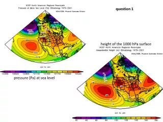
question 1 height of the 1000 hPa surface pressure (Pa) at sea level
start with pressure at 1500 m MSL then use hydrostatic balance to estimate the height of the 855 mb surface at B then draw the 855 mb isobar use the same method to estimate the height of the 850 mb surface at A and to draw the 850 mb isobar Note: density variations are secondary – to a first order, density (thickness) can be assumed constant. height 850 855 high low A B Pressure decreases with height at about 10 mb every 100 m
question 2 DZ1000,500 Z500 Jan 2010 Jan 2010 DZ1000,500 Z500 Jul 2010 Jul 2010
question 3 sea-level pressure Jan 2010 Jul 2010 NH winter summer SH
Schematic zonal-mean cross section (after Palmen & Newton) ITCZ
The Palmen-Newton model has three meridional circulation cells in each hemisphere Note that the three-cell pattern ignores seasonal variation and land-sea contrast.
How strong are the meridional cells? (zonal mean) Jan NH winter Hadley Ferrel note the broad belt of subsidence (12-52ºN) in winter and the broad belt of ITCZ ascent (0-30ºN) in summer. ITCZ • In the NH winter, over continents, the northern Hadley cell rising branch crosses the Equator into the SH ITCZ, • and its sinking branch extends between 12-50ºN July NH summer Ferrel NH Hadley SH Hadley Effectively ascent dominates in the summer hemisphere, and sinking in the winter hemisphere, and the Hadley cell that straddles the equator is the strongest. ITCZ
Structure of SLP, winds, temperatureseasonal march of sea level pressure and sfc winds • northern oceans: • polar lows: Aleutian, Icelandic • subtropical highs: Pacific, Bermuda • northern continents: • - winter highs: Siberian, Intramtn • - summer lows: Pakistan, Sonoran • southern oceans: • - circumpolar (southern) low • - subtropical highs (3 oceans) observations: - A see-saw SLP variation dominates over the northerncontinents, with highs in winter and lows in summer. The seasonal variation of the polar lows and subtropical highs over the northern oceans is also large, and is in opposition to SLP variations over land at corresponding latitudes. - The southern hemisphere is far more zonally symmetric. - Note the extremely low SLP around the Antarctic ice dome.
seasonal march of surface air temperature note that the amplitude of the annual temperature range is higher at: - higher latitudes - over land rather than over water [this does NOT occur in terms of net radiation Rn] - over large land masses, especially their eastern side
question 4 Speed for 1 = 4.1 m/s Speed for 2 = 16.4 m/s Speed for 3 = 10.8 m/s