Efficient Storage and Querying for Multidimensional Databases
Explore challenges in representing multidimensional data, indexing, and querying for efficient storage. Examples include time-series and image data, with new approaches for complex data sets like graphs and Immersidata. Learn about key challenges in storing and indexing data, executing spatial and temporal queries, and mining multidimensional data. Discover methods for aggregation, clustering, classification, and outlier detection.

Efficient Storage and Querying for Multidimensional Databases
E N D
Presentation Transcript
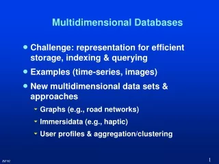
Multidimensional Databases • Challenge: representation for efficient storage, indexing & querying • Examples (time-series, images) • New multidimensional data sets & approaches • Graphs (e.g., road networks) • Immersidata (e.g., haptic) • User profiles & aggregation/clustering
Challenges • Storing multidimensional data (matrix vs. relations) • Indexing multidimensional data (R-tree) • Queries • Search for similar objects (similarity search)[ICDE’00,ICME’00] • Spatial and temporal queries [IDEAS’00,ACM-GIS’01,KAIS’02] • Multidimensional data mining • Aggregation [EDBT’02,PODS’02] • Clustering[ACM-MMj’02] • Classification [INFORMS’02] • Finding outliers [SSDBM’01]
$price $price f1 e.g., std f2 f5 f (S1) g (S1) 1 1 365 365 day day g (Sn) f (Sn) f3 e.g., avg f4 • A point in 5 dimensions • transformation-based: • FFT, Wavelet [SSDBM’00, 01] • A point in 365 dimensions • (computationally complex) • A point in 2 dimensions • (not accurate enough) Stock Prices S1 Sn
R 255 0 Red Green Blue Red Green Blue . . . 208 125 100 80 100 210 G B More accurate Images Color Histograms j 1 j 2 j 9 j 3 j 8 j 7 j 4 j 5 j 6 Web Navigations Angle Sequences = [j1,j2,j3,j4,j5,j6,j7,j8,j9] P1 P2 P3 P4 P5 … 3 0 8 7 (Hit) Feature Vectors [RIDE’97 … WebKDD’01] More Similarity Search & Clustering C Shapes [ICDE’99 … ICME’00]
On-Line Analytical Processing (OLAP) Market-Relation • Multidimensional data sets: • Dimension attributes (e.g., Store, Product, Date) • Measure attributes (e.g., Sale, Price) • Range-sum queries • Average sale of shoes in CA in 2001 • Number of jackets sold in Seattle in Sep. 2001 • Tougher queries: • Covariance of sale and price of jackets in CA in 2001 (correlation) • Variance of price of jackets in 2001 in Seattle Store Location Date Sale Product Price LA Shoes Jan. 01 $21,500 $85.99 NY Jacket June 01 $28,700 $45.99 . . . . . . . . . . . . . . . Avg (sale) s(d <in> 2001) Too Slow! s(s <in> CA) s(p=shoe) Market-Relation
Query: Sum(salary) when (25 < age < 40) and (55k < salary < 150k) Query: Sum(salary) when (25 < age < 40) and (55k < salary < 150k) Example Solution (Pre-computation): Prefix-sum [Agrawal et. al 1997] Salary Age Salary $150k $100k $120k $40k $55k $65k • $50k • $55k • $58k • $100k • $130k • 57 $120k 0 25 40 Age 50 60 • Issues: • Measure attribute should be pre-selected • Aggregation function should be pre-selected (sum or count) • Updates are expensive (need re-computation) 80 Result: I – II – III + IV
Spatial & Temporal Data Complex Queries [ACM-GIS’01, VLDB’01] • Data types: • A point: <latitude, longitude, altitude> or <x, y, z> • A line-segment: <x1, y1, x2, y2> • A line: sequence of line-segments • A region: A closed set of lines • Moving point: <x, y, t> (e.g., car, train, …) • Changing region: <region, value, t> (e.g., changing temperature of a county) • Queries: • Rivers <intersect> Countries • Hospitals <in> Cities • Taxi <within> 5km of Home • <in the next> 10 min • Experiments <overlap> BrainR [Visual’99]
Station Spatial & Temporal Data & Queries Data types: • A point: <latitude, longitude, altitude> or <x, y, z> • A line-segment: <x1, y1, x2, y2> • A line: sequence of line-segments • A region: A closed set of lines • Moving point: <x, y, t> (e.g., objects, car, train, …) Queries: • Molecules <intersect> Microbes • Train-stations <in> Cities • Round objects <within> 5cm of Hand <in the next> 10 s • Number of distractions in <south-east> of subject
What is nearest? In road network (or a graph) is “shortest path” which is complex to compute in real-time for all points of interests • Approach: embed graph into high dimensional space where computationally simple Minkowski metrics (e.g., Euclidean) can approximate real distances [ACM-GIS’02?] 2-D Space n-D Space Embedding Techniques (e.g., Lipschitz) A A B C C B Spatial & Temporal Data & Queries … • K Nearest Neighbor queries: find the k nearest objects to a query point (5 closest hospitals to my car)
Immersidata and Mining Queries [CIKM’01, UACHI’01]
Immersidata and Mining Queries … … Subject-2 Subject-3 Subject-n … SVD SVD SVD SVD L: A dynamic sign, e.g., ASL colors Subject-1
Clusters Item Database User Profiles User 1 User 2 User 3 Fuzzy Aggregation User 4 User 5 User 6 User U-6 Cluster Wish-list User U-5 User U-4 0.87 0.83 User U-3 0.72 User U-2 0.61 User U-1 0.47 User U User Profiles & Clustering Offline Processes PPED Similarity Measure and Clustering Favorite Features (Rock= High Classical= Low Pop= Low Rap= High) Voting
Clusters Cluster Wish-lists User Wish-List 0.87 0.87 0.87 0.83 0.83 0.83 0.72 0.72 0.72 PPED Similarity Measure 0.87 0.61 0.61 0.61 0.83 0.47 0.47 0.47 0.82 0.79 0.72 0.70 0.68 Fuzzy Aggregation 0.65 A List of Similarity Values 0.63 0.65 0.32 0.79 0.61 0.54 0.47 0.42 User Profiles & Clustering Online Processes Current User’s Profile
