Download
1 / 35
360 likes | 648 Vues
6.5 DESCRIPTIVE STATISTICS FOR GROUPED DATA. If there were 30 observations of weekly sales then you had all 30 numbers available to you. When you are trying to solve a problem by analyzing data, this is the best situation to be in. You have what is known as raw or ungrouped data .

E N D
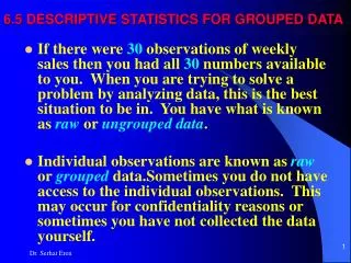
6.5 DESCRIPTIVE STATISTICS FOR GROUPED DATA • If there were 30 observations of weekly sales then you had all 30 numbers available to you. When you are trying to solve a problem by analyzing data, this is the best situation to be in. You have what is known as raw or ungrouped data. • Individual observations are known as raw or grouped data.Sometimes you do not have access to the individual observations. This may occur for confidentiality reasons or sometimes you have not collected the data yourself. Dr. Serhat Eren
6.5 DESCRIPTIVE STATISTICS FOR GROUPED DATA • if you are using secondary data, and much of the data published on the Web are unavailable as raw data. Thus, often the only thing available to you is what is known as grouped data. • For example, suppose you wished to compare the salaries of managers in your organization to national values. The human resource manager may not wish to share individual salary values with you but might give you information in the following form: Dr. Serhat Eren
Time Frequency 0 < x $30,000 30,000 < x 60,000 60,000 < x 90,000 1 8 3 6.5 DESCRIPTIVE STATISTICS FOR GROUPED DATA • Grouped dataare data that are available only as a frequency distribution. The individual observations are not accessible. Dr. Serhat Eren
6.5 DESCRIPTIVE STATISTICS FOR GROUPED DATA 6.5.1 Measures of the Center for Grouped Data • There are three measures of the center: the mean, the median, and the mode. • First consider how to estimate the mean of the data set when you have grouped data. • For example, consider the amount of time, in minutes, people occupy a table in a particular restaurant. The manager is interested in the center or the typical length of time that the table is occupied. She has only the following frequency table from 32 observations: Dr. Serhat Eren
Time Frequency 25.0 < x 35.0 35.0 < x 45.0 45.0 < x 55.0 55.0 < x 65.0 65.0 < x 75.0 75.0 < x 85.0 85.0 < x 95.0 5 2 4 3 11 3 4 6.5 DESCRIPTIVE STATISTICS FOR GROUPED DATA • Remember that to calculate the mean you sum all the data and divide by the sample size. Dr. Serhat Eren
6.5 DESCRIPTIVE STATISTICS FOR GROUPED DATA • But for grouped data you cannot sum the actual data because you don't have them. So, you have to estimate what the values might sum to for each interval. • Consider the 5 observations that fall in the first interval between 25 and 35 minutes. • We need a way to estimate the sum of those 5 values to begin our estimation of the mean. Dr. Serhat Eren
6.5 DESCRIPTIVE STATISTICS FOR GROUPED DATA • It seems reasonable to use the middle of the interval as our best "guess" of the actual values m the class. So, you must first find the midpoint of each class. • In this dataset, the 5 values for table times that fall between 25 and 35 min are assumed to be spread evenly throughout the interval so that the middle value of 30 minutes is a good representation of the data in that interval. Dr. Serhat Eren
6.5 DESCRIPTIVE STATISTICS FOR GROUPED DATA • Since there are 5 of them, you multiply the midpoint of 30 by the frequency of 5 to get the contribution to the sum for that interval. This is like adding 5 values of 30 together. • This process is repeated for each interval and then the sums are added together and divided by the sample size. • The details are shown in the next example. Dr. Serhat Eren
6.5 DESCRIPTIVE STATISTICS FOR GROUPED DATA • This procedure is summarized in the steps below. It gives you a good estimate of the mean when the data are in fact evenly spread out throughout the interval. • Step 1. Find the midpoint of each class. Call it mj. • Step 2. Multiply the midpoint by the class frequency, fj, to yield fjmj. • Step 3. Add up all the interval sums found in step 2. • Step 4. Divide the sum from step 3 by the sample size, n. Note that the sample size is the sum of all the frequencies. Dr. Serhat Eren
6.5 DESCRIPTIVE STATISTICS FOR GROUPED DATA • The formula for estimating the mean from grouped data is thus Dr. Serhat Eren
6.5 DESCRIPTIVE STATISTICS FOR GROUPED DATA • Recall that the median is the data value of the middle observation in an ordered set of data; thus it is the value at or below which half (50%) of the data values fall. • So to find the median for grouped data we need to find the midpoint of the interval that contains the data value whose cumulative relative frequency is 0.50. Dr. Serhat Eren
6.5 DESCRIPTIVE STATISTICS FOR GROUPED DATA 6.5.1 Measures of the Center for Grouped Data • Recall that the mode is the data value that has the highest frequency of occurrence in the sample. • Using this definition, it is easy to see that the modal class is the class interval in the frequency distribution that has the highest frequency. • The estimate of the mode is then the midpoint of the modal class. Dr. Serhat Eren
6.5 DESCRIPTIVE STATISTICS FOR GROUPED DATA 6.5.2 Measures of Dispersion for Grouped Data • Clearly with grouped data the sample range can be estimated by taking the difference between the upper value of the last class and the lower value of the first class. • In order to adapt the formula for the sample variance for use with grouped data, we need to take the same approach that we used for estimating the sample mean for grouped data. Dr. Serhat Eren
6.5 DESCRIPTIVE STATISTICS FOR GROUPED DATA • In particular, we need to adapt the formula for the sample variance shown below to accommodate the fact that we no longer have the individual data values represented by xiin the formula Dr. Serhat Eren
6.5 DESCRIPTIVE STATISTICS FOR GROUPED DATA • The following formula and steps for estimating the sample variance for grouped data. Dr. Serhat Eren
6.5 DESCRIPTIVE STATISTICS FOR GROUPED DATA • Step 1. Find the midpoint of each class. Call it mj. • Step 2. Subtract the estimate of the sample mean,from each class midpoint. Square the difference. • Step 3. Multiply the result of step 2 by the class frequency. • Step 4. Add up the results of step 3 for all classes. • Step 5. Divide the sum from step 4 by one less than the sample size, n - 1. Dr. Serhat Eren
6.6 MEASURES OF RELATIVE STANDING 6.6.1 Percentiles • It is useful in some real situations to know what data value in a sample has a certain percentage of the sample above or below it. • This measure is known as the percentile of the data. • The pth percentile of a data set is the value that has p% of the data at or below it. Dr. Serhat Eren
6.6 MEASURES OF RELATIVE STANDING • Two questions can be asked involving percentiles: • What value has p%of the data at or below it? • What is the percentile rank of a particular data value? • The first question involves finding either a particular percentile or set of percentiles, such as the deciles (10%, 20%, . . . ,90%). The second question involves finding the percentile rank of a particular value in a data set. Dr. Serhat Eren
6.6 MEASURES OF RELATIVE STANDING • The percentile rankof a value is the percentage of the data in the sample that are at or below the value of interest. • This measure allows you to determine the relative standingof an observation in a set of data. • To find the percentile rank of an observation, the data must be put in numerical order. Dr. Serhat Eren
6.6 MEASURES OF RELATIVE STANDING • The percentile rank, P, is then found by b= the number of data values below the value of interest e= the number of data values equal to the value of interest n= the sample size Dr. Serhat Eren
6.6 MEASURES OF RELATIVE STANDING 6.6.2 Quartiles • There are certain percentiles that are used frequently. These percentiles are the 25th percentile and the 75th percentile, also known as the first and third quartiles. • The first quartile, Ql,is the value in the sample that has 25% of the data at or below it. • The third quartile, Q3, is the value in the sample that has 75% of the data Dr. Serhat Eren
6.6 MEASURES OF RELATIVE STANDING • Since percentiles and quartiles are order statistics, finding them requires that the data set be sorted from lowest to highest, • Step 1: Put the data set in order and find the median of the data. • Step 2: Take the lower half of the data and find the median of the lower half of the data. This value will be the first quartile, Q1. • Step 3: Take the upper half of the data and find the median of the upper half of the data. This value will be the third quartile, Q3. Dr. Serhat Eren
6.6 MEASURES OF RELATIVE STANDING 6.6.3 Displaying the Data Using Box-plots • A box-plotor box and whisker diagramis a graphical display that uses summary statistics to display the distribution of a set of data.A box-plot summarizes a sample using the quartiles and the median. • If you look at the first and third quartiles of a sample, Q1and Q3, you see that 50% of the data in the sample fall between these two values. The distance between these two values is called the interquartile range (IQR). Dr. Serhat Eren
6.6 MEASURES OF RELATIVE STANDING • The interquartile range(IQR) is the difference between the third and first quartilesQ3 - Q1. • Figure 6.6 provides a partial picture of the data set. • To complete the description with the empirical rule we used two additional intervals, ±2 and ±3. Dr. Serhat Eren
6.6 MEASURES OF RELATIVE STANDING 6.6.4 Using a Box-plot to Identify Outliers • Sample data that fall between the inner and outer fences are called possible outliers, while data values that fall beyond the outer fences are called probable outliers. • If you are having trouble figuring out the difference betweenprobableand possible, think about the difference in your reaction when I tell you, "It is possiblethat you will pass this course" vs. "It is probablethat you will pass this course." Dr. Serhat Eren