Download
1 / 22
220 likes | 337 Vues
Six-dimensional weak-strong simulations of head-on compensation in RHIC. Y. Luo , W. Fischer Brookhaven National Laboratory, USA ICFA Mini-workshop on Beam-Beam Effects in Hadron Colliders, March 18-22, 2013, CERN . Content. Introduction Dynamic Aperture Calculation

E N D
Six-dimensional weak-strong simulations of head-on compensation in RHIC Y. Luo, W. Fischer Brookhaven National Laboratory, USA ICFA Mini-workshop on Beam-Beam Effects in Hadron Colliders, March 18-22, 2013, CERN
Content • Introduction • Dynamic Aperture Calculation • Particle Loss Rate Calculation • Sensitivity Study • Summary Here we focus on weak-strong beam-beam simulation results for RHIC head-on beam-beam compensation. For strong-strong simulation results, please see S. White’s talk.
Introduction • To further increase Luminosity in the RHIC polarized proton run we are continuing to increase bunch intensity and decrease β*. • With the newly upgraded polarized proton source, the maximum bunch intensity at store in RHIC will increase from currently 1.7 × 10¹¹ up to 3.0 × 10¹¹ . The beam-beam parameter will exceed 0.025. • Current RHIC working point is constrained between 2/3 and 7/10. There is no enough tune space between 2/3 and 7/10 to hold the large beam-beam tune spread when the proton bunch intensity is higher than 2.0 × 10¹¹. Tune footprints with Np= 2.0 × 10¹¹ with beam-beam parameter 0.02.
Head-on Beam-beam compensation • Head-on beam-beam compensation (BBC) has been adopted in RHIC for beam-beam tune spread and nonlinear beam-beam resonance driving term (RDT) compensations. • Two electron lenses (e-lenses) have been installed on either side of IP10, one for compensation in Blue ring, and one for Yellow ring. Proton beams are separated vertically in e-lenses. • The electron beam should have same transverse profile and beam size as the proton bunches at e-lenses for best cancellation of BB effects. Layout RHIC BBC RHIC e-lenses installation
Weak-strong BB simulation code • Code : SimTrack ( by Y. Luo ) - C++ library: flexible, manageable - 4th order symplectic integration for magnets - 6-D synch-beam map for p-p beam-beam - 4-D beam-beam kickers for e-p beam-beam - element-by-element tracking - nonlinear interaction region magnet fields used • Code benchmarking with other codes - optics benchmarked with TRACY-II ( J. Bengtsson) - 6-D beam-beam benchmarked with BBSIMC ( Y-J. Kim, T. Sen) - particle loss compared with BBSIMC, LifeTrac ( A. Valishev)
Tune footprints w/o BBC • Plots below show the tune footprints without / with beam-beam compensation. In this example, we used bunch intensity 2.5× 10¹¹ , normalized emittance 15 Pi mm.mrad. • We define full beam-beam compensation (FBBC) and half head-on beam-beam compensation (HBBC) to compensate full and half of total beam-beam tune shift . • Partial head-on beam-beam compensation is to be used in RHIC. Np= 2.5× 10¹¹ , half compensation Np= 2.5× 10¹¹, no compensation
Dynamic Aperture Calculation • In this section, we present DA results: • without and with BBC • parameter scans • - phase advances between IP and e-lenses • second order chromaticity correction • Dynamic aperture has been used to determine single particle’s stability in RHIC and results qualitatively agreed well with observations.
DA with and without compensation • In the following simulation, zero-amplitude tunes are always set to (0.67, 0.68) under different BB conditions. • Left plot shows that DA without BBC, with FBBC, and HBBC in the scan of proton bunch intensity. Simulation results show that HBBC improves DA when Np > 2.5× 10¹¹ . FBBC reduces DA for all bunch intensities. • Explanation: HBBC moves the tune spread away from 7/10 resonance line. • Explanation: FBBC compensates almost all of BB tune spread, its tune footprint is every irregular due to Qx=2/3 resonance . FBBC also gives largest beam-beam RDTs.
Compensation strength • We define compensate strength: • Here we adjust N*e to change κ. • Simulation results show that for all of the bunch intensities, DA begins to drop sharply when compensation strength exceeds 0.7. • The optimized compensation strength for Np= 2.5× 10¹¹ and 3.0× 10¹¹ is around 0.5-0.6.
Phase adjustment and Q’’ correction • Two shunt power supplies are added to the main arc quadrupoles between IP8 and IP10 to adjust the phase advances between IP8 and e-lens to be K * π for cancellation of IP8 ‘s contributions to beam-beam RDTs with the e-lens . • Global second order chromaticity correction is applied to improve the off-momentum dynamic aperture. • Simulation results show that the phase adjustment between IP8 and e-lens, and second order chromaticity correction improve the dynamic aperture of HBBC.
Electron beam size HBBC FBBC • A 2-D scan of electron current and electron beam size shows that the maximum DA with head-on beam-beam compensation is around half beam-beam compensation with the electron beam size slightly larger than the proton beam’s.
Tune scan with compensation • With BBC, the tune footprint becomes smaller and therefore it is possible to scan the proton working point between 2/3 and 7/10 to maximize DA. • Simulation shows that HBBC prefers lower tunes while FBBC prefers higher tunes. The maximum DA of FBBC is smaller than that of HBBC in the tune scan. HBBC tune scan FBBC tune scan
Particle Loss Rate Calculation • In this section, we present multi-particle long-term tracking results with head-on beam compensation in RHIC: • challenges in multi-particle tracking • new approaches & algorithms • some particle loss rate calculation
Challenges in multi-particle tracking • Beam-beam study tools - single particle tracking: tune diffusion, action diffusion, dynamic aperture (DA), etc. - multi-particle tracking: beam lifetime, emttance growth • Dynamic aperture versus lifetime - DA doesn’t give information about emittance - DA is not direct connected beam lifetime - online measurement of DA is tedious - beam decay, emittances, luminosity are measured on line • Challenges in multi-particle tracking - Limited computing time : have to reduce particle number, tracking turns - Limited resolution in tracking results: for example, for RHIC multi-particle tracking, 2 ×10⁶ turns ( 24 seconds) to detect 1% / hour beam decay resolution: 0.007% in particle loss to detect 20% emittance increase over 10 hour resolution: 0.02% in emittance
Techniques & Algorithms • For limited multi-particle number (4800), we use 1) weighted particle distribution ( LifeTrac) • 2) Hollow Gaussian particle distribution ( BBSIMC) • For hollow Gaussian distribution, only track particles with amplitudes above certain transverse and longitude boundaries. Particles inside that boundaries are considered stable and don’t track. • For example, HBBC with bunch intensity Np= 2.5× 10¹¹ , 4800 macro-particles, over 2× 10⁶ turns. Following table shows the calculated beam decays with three initial particle distributions: Weighted Gaussian Hollow Gaussian
Particle loss rates Bunch intensity 2.5× 10¹¹ Bunch intensity 3.0× 10¹¹ 1.5%/hour 15%/hour • Multi-particle simulation results confirm the results from DA tracking: HBBC improves the beam lifetime of half beam-beam compensation. And the phase adjustment between IP8 and e-lens, and second order chromaticity correction further increase the proton beam lifetime.
Sensitivity Study • In this section, we present the sensitivity of head-on beam-beam compensation on the beam imperfections and beam noises: • truncated Gaussian electron distribution • offsets between electron and proton beams • noises in electron beam current
Truncated Gaussian Tail • RHIC e-lens gun design and real measurement show that the electron beam has a Gaussian tail cut off at 2.8 . This is determined by electric field distribution on cathode. • Simulation shows that Gaussian tail cut at 2.8 from the current electron gun design is acceptable.
Offset of electron and proton beams • Over-lapping of the electron and proton beams in the e-lens plays a crucial role in the head-on beam-beam compensation. • Based on particle loss rate calculations, we set the static offset error tolerance to be 30 μm which is a tenth of a rms beam size in the e-lens, and the random offset tolerance to be 9 μm which requires stability of bending magnet’s power supply better than 0.01%. Static offset Random offset
Noise in electron current • Due to the instability of the power supplies of the electron gun, there is noise in the electron beam current. • Based on particle loss rate calculation, we require that the stability of the power supplies of the electron gun should be better than 0.1% .
Summary • We presented the 6-D weak-strong simulation results for the head-on beam-beam compensation in RHIC. Dynamic aperture, particle loss rate, and sensitivity are calculated. • Calculated dynamic aperture and particle loss rate show that half beam-beam compensation improves proton beam’s beam lifetime. And phase advance adjustment between IP8 and e-lens, and second order chromaticity correction further increase the proton beam lifetime. • In the following months we will repeat simulations with the real RHIC e-lens lattices and focus on the e-lens lattice optimization, nonlinear corrections with head-on beam-beam compensation.
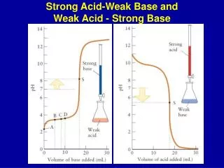


![pH = -log [H + ] . Strong Acid . Strong base . Weak Acid. Weak Base.](https://cdn3.slideserve.com/6574453/slide1-dt.jpg)