Download
1 / 46
500 likes | 789 Vues
Dip. di Ingegneria Industriale - Università di Parma Parco Area delle Scienze 181/A, 43100 Parma – Italy angelo.farina@unipr.it www.angelofarina.it. ACOUSTICS part – 3 Sound Engineering Course. Angelo Farina. The Sound Intensity meter. Euler equation: the sound intensity probe.

E N D
Dip. di Ingegneria Industriale - Università di Parma Parco Area delle Scienze 181/A, 43100 Parma – Italy angelo.farina@unipr.it www.angelofarina.it ACOUSTICSpart – 3 Sound Engineering Course Angelo Farina
Euler equation: the sound intensity probe A sound intensity probe is built with two amplitude and phase matched pressure microphones: The particle velocity signal is obtained integrating the difference between the two signals:
Euler’s Equation Connection between sound pressure and particle velocity; it is derived from the classic Newton’s first law ( F = m · a ): It allows to calulate particle velocity by time-integrating the pressure gradient: The gradient is (approximately) known from the difference of pressure sampled by means of two microphones spaced a few millimeters (SOund Intensity probe).
Sound Intensity probe (1) The Sound Intensity is: Where both p and v can be derived by the two pressure signals captured by the two microphones
Sound Intensity Probe: errors Phase Mismatch Error due to a phase error of 0.3° in a plane propagating wave Finite-Differences Error of a sound intensity probe with 1/2 inch microphones in the face-to-face configuration in a plane wave of axial incidence for different spacer lengths: 5 mm (solid line); 8.5 mm (dashed line); 12 mm (dotted line); 20 mm (long dashes); 50 mm (dash-dotted line)
Omnidirectional microphones ISO3382 recommends the usage of omni mikes of no more than 13mm These are the same microphones usually employed on sound level meters: Sound Level Meter(records a WAV file on the internal SD) (left) Measurement-grade microphone and preamplifier (to be connected to a sound card)(right)
Spatial analysis by directive microphones The initial approach was to use directive microphones for gathering some information about the spatial properties of the sound field “as perceived by the listener” Two apparently different approaches emerged: binaural dummy heads and pressure-velocity microphones: Binaural microphone (left) and variable-directivity microphone (right)
Test with binaural microphones Cheap electret mikes in the ear ducts
Capturing Ambisonics signals A tetrahedrical microphone probe was developed by Gerzon and Craven, originating the Soundfield microphone
Soundfield microphones The Soundfield microphone allows for simultaneous measurements of the omnidirectional pressure and of the three cartesian components of particle velocity (figure-of-8 patterns)
Directivity of transducers Soundfield ST-250 microphone
Alternative A-format microphones At UNIPR many other 1st-order Ambisonics microphones are employed (Soundfield TM, DPA-4, Tetramic, Brahma) 16
Portable, 4-channels microphone A portable digital recorder equipped with tetrahedrical microphone probe: BRAHMA
The D’Alambert equation The equation comes from the combination of the continuty equation for fluid motion and of the 1st Newton equation (f=m·a). In practive we get the Euler’s equation: now we define the potential F of the acoustic field, which is the “common basis” of sound pressure p and particle velocity v: Subsituting it in Euler’s equation we get:: D’Alambert equation Once the equation is solved and F is known, one can compute p and v.
Free field propagation: the spherical wave Let’s consider the sound field being radiated by a pulsating sphere of radius R: v(R) = vmax ei ei = cos() + i sin() Solving D’Alambert equation for r > R, we get: Finally, thanks to Euler’s formula, we get back pressure: k = w/cwave number
Free field: proximity effect From previous formulas, we see that in the far field (r>>l) we have: But this is not true anymore coming close to the source. When r approaches 0 (or r is smaller than l), p and v tend to: This means that close to the source the particle velocity becomes much larger than the sound pressure.
Free field: proximity effect The more a microphone is directive (cardioid, hypercardioid) the more it will be sensitive to the partcile velocty (whilst an omnidirectional microphone only senses the sound pressure). So, at low frequency, where it is easy to place the microphone “close” to the source (with reference to l), the signal will be boosted. The singer “eating” the microphone is not just “posing” for the video, he is boosting the low end of the spectrum...
Free field: Impedance If we compute the impedance of the spherical field (z=p/v) we get: When r is large, this becomes the same impedance as the plane wave (r ·c). Instead, close to the source (r < l), the impedance modulus tends to zero, and pressure and velocity go to quadrature (90° phase shift). Of consequence, it becomes difficult for a sphere smaller than the wavelength l to radiate a significant amount of energy.
Free field: energetic analysis, geometrical divergence The area over which the power is dispersed increases with the square of the distance.
Free field: sound intensity If the source radiates a known power W, we get: Hence, going to dB scale:
Free field: propagation law • A spherical wave is propagating in free field conditions if there are no obstacles or surfacecs causing reflections. • Free field conditions can be obtained in a lab, inside an anechoic chamber. • For a point source at the distance r, the free field law is: • Lp = LI= LW - 20 log r - 11 + 10 log Q (dB) • where LW the power level of the source and Q is the directivity factor. • When the distance r is doubled, the value of Lp decreases by 6 dB.
Free field: directivity (1) • Many soudn sources radiate with different intensity on different directions. Hence we define a direction-dependent “directivity factor” Q as: • Q = I / I0 • where Iè is sound intensity in direction, and I0is the averagesound intensity consedering to average over the whole sphere. • From Q we can derive the direcivity index DI, given by: • DI = 10 log Q (dB) • Q usually depends on frequency, and often increases dramatically with it. Iq I0
Free Field: directivity (2) • Q = 1 Omnidirectional point source • Q = 2 Point source over a reflecting plane • Q = 4 Point source in a corner • Q = 8 Point source in a vertex
Line Sources Many noise sources found outdoors can be considered line sources: roads, railways, airtracks, etc. • Geometry for propagation from a line source to a receiver • in this case the total power is dispersed over a cylindrical surface: In which Lw’ is the sound power level per meter of line source
Coherent cylindrical field • The power is dispersed over an infinitely long cylinder: L r In which Lw’is the sound power level per meter of line source
“discrete” (and incoherent) linear source Another common case is when a number of point sources are located along a line, each emitting sound mutually incoherent with the others: • Geomtery of propagation for a discrete line source and a receiver • We could compute the SPL at teh received as the energetical (incoherent) summation of many sphericla wavefronts. But at the end the result shows that SPL decays with the same cylndrical law as with a coherent source: The SPL reduces by 3 dB for each doubling of distance d. Note that the incoherent SPL is 2 dB louder than the coherent one!
Example of a discrete line source: cars on the road Distance a between two vehicles is proportional to their speed: In which V isspeed in km/h and Nis the number of vehiclespassing in 1 h • The sound powerlevelLWp of a single vehicleis: • Constant up to 50 km/h • Increases linearly between 50 km/h and 100 km/h (3dB/doubling) • Above 100 km/h increases with the square of V (6dB/doubling)
Example of a discrete line source: cars on the road Hence there is an “optimal” speed, which causes the minimum value of SPL, which lies around 70 km/h Modern vehicles have this “optimal speed” at even larger speeds, for example it is 85 km/h for the Toyota Prius
Free field: excess attenuation • Other factors causing additional attenuation during outdoors progation are: • air absorption • absorption due to presence of vegetation, foliage, etc. • metereological conditions (temperature gradients, wind speed gradients, rain, snow, fog, etc.) • obstacles (hills, buildings, noise barriers, etc.) • All these effects are combined into an additional term L, in dB, which is appended to the free field formula: • LI = Lp = LW - 20 log r - 11 + 10 log Q - L (dB) • Most of these effects are relevant only at large distance form the source. The exception is shielding (screen effect), which instead is maximum when the receiver is very close to the screen
Excess attenuation: temperature gradient Shadow zone
Excess attenuation: air absorption Air absorption coefficients in dB/km (from ISO 9613-1 standard) for different combinations of frequency, temperature and humidity:
Noise screens (1) • A noise screen causes an insertion lossL: • L = (L0) - (Lb) (dB) • where Lb and L0 are the values of the SPL with and without the screen. • In the most general case, there arey many paths for the sound to reach the receiver whne the barrier is installed: • diffraction at upper and side edges of the screen (B,C,D), • passing through the screen (SA), • reflection over other surfaces present in proximity (building, etc. - SEA).
Noise screens (2): the MAEKAWA formulas • If we only consider the enrgy diffracted by the upper edge of an infinitely long barrier we can estimate the insertion loss as: • L= 10 log (3+20 N) for N>0 (point source) • L = 10 log (2+5.5 N) for N>0 (linear source) • where N is Fresnel number defined by: • N = 2 / = 2 (SB + BA -SA)/ • in which is the wavelength and is the path difference among the diffracted and the direct sound.
Noise screens (3): finite length • If the barrier is not infinte, we need also to soncider its lateral edges, each withir Fresnel numbers (N1, N2), and we have: • L = Ld - 10 log (1 + N/N1 + N/N2) (dB) • Valid for values of N, N1, N2 > 1. • The lateral diffraction is only sensible when the side edge is closer to the source-receiver path than 5 times the “effective height”. heff R S
Noise screens (4) • Analysis: • The insertion loss value depends strongly from frequency: • low frequency small sound attenuation. • The spectrum of the sound source must be known for assessing the insertion loss value at each frequency, and then recombining the values at all the frequencies for recomputing the A-weighted SPL. SPL (dB) No barrier – L0 = 78 dB(A) Barrier – Lb = 57 dB(A) f (Hz)