Download
1 / 23
260 likes | 553 Vues
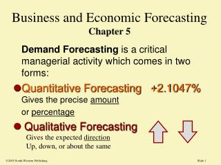
Business and Economic Forecasting. Mohammad Arief. Overview. Demand Forecasting is a critical managerial activity. Qualitative. Quantitative. Gives the expected direction Up, down, or about the same. Gives the precise amount or percentage. THE SIGNIFICANCE OF FORECASTING.

E N D
Business and Economic Forecasting Mohammad Arief
Overview Demand Forecasting is a critical managerial activity Qualitative Quantitative • Gives the expected direction Up, down, or about the same Gives the precise amountor percentage
THE SIGNIFICANCE OF FORECASTING Uncertainty Conditions limited Predicting changes in cost, price, sales, and interest rates Accurate forecasting can help develop strategies to promote profitable trends and to avoid unprofitable ones
SELECTING A FORECASTING TECHNIQUE The forecasting technique used in any particular situation depends on a number of factors. • Hierarchy of Forecasts • Criteria Used to Select a Forecasting Technique • Evaluating the Accuracy of Forecasting Models
Hierarchy of Forecasts • The highest level of economic aggregation that is normally forecast is that of the national economy (GDP, interest rates, inflation, etc). • Sectors of the economy (durable goods) • Industry forecasts(all auto manufacturers) • Firm forecasts (Ford Motor Company) • Product forecasts (The Ford Focus)
Forecasting Criteria The choice of a particular forecasting method depends on several criteria: • costsof the forecasting method compared with its gains • complexityof the relationships among variables • timeperiod involved • accuracyneeded in forecast • lead time between receiving information and the decision to be made
Accuracy of Forecasting • The accuracy of a forecasting model is measured by how close the actual variable, Y, ends up to the forecasting variable, Y. • Forecast error is the difference. (Y - Y) • Models differ in accuracy, which is often based on the square root of the average squared forecast error over a series of N forecasts and actual figures • Called a root mean square error, RMSE. • RMSE = { (Y - Y)2 / N } ^ ^ ^ The smaller the value of the RMSE, the greater the accuracy
ALTERNATIVE FORECASTING TECHNIQUES • Deterministic trend analysis • Smoothing techniques • Barometric indicators • Survey and opinion-polling techniques • Macroeconometric models • Stochastic time-series analysis
1. Deterministic trend analysis • Time-series data, A sequence of the values of an economic variable at different points in time. • Cross-sectional data An array of the values of an economic variable observed at thesame time, like the data collected in a census across many individuals in the population. These are long-run trends that cause changes in an economic data series Secular trends These are major expansions and contractions in an economicseries that are usually greater than a year in duration Cyclical variations Seasonal variations during a year tend to be more or lessconsistent from year to year. Seasonal effects an economic series may be influenced by random factors that are unpredictable Random fluctuations
Secular trends (Trend Sekuler) • Forecasting model trend sekuler dilakukan dengan menarik garis secara kasar atau serampang mengikuti kecenderungan permintaan yang terjadi secara siklus dari tahun ke tahun.
Cyclical variations (Fluktuasi Siklus) • Siklus perubahan atau naik turunnya volume permintaan selama tahun-tahun yang telah lalu dan yang akan dating,kita tarik kecenderungannya tentu disebabkan atau dipengaruhi oleh sejumlah faktor yang secara periodik dan tetap harus ada atau terjadi selam periode tahunan yang akan datang. • Biasanya siklus bisa kita duga sebelumnya bahwa dengan datangnya permintaan yang meningkat pada periode tertentu sudah bisa kita prediksi kejadiannya.
Seasonal effects(Metode Variasi Musim) • Melakukan prakiraan volume permintaan konsumen di waktu-waktu yang akan datang dapat didasarkan pada gelombang musiman yang melekat pada kultur budaya atau kebiasaan dari masyarakat. • Tetapi dapat juga karena faktor sifat dan keadaan alam yang melekat pada iklim atau cuaca. Misalnya produksi musim semi, gugur, dan musim hujan bahkan musim kemarau.
Random fluctuations (Fluktuasi Siklus) • Siklus perubahan atau naik turunnya volume permintaan selama tahun-tahun yang telah lalu dan yang akan dating,kita tarik kecenderungannya tentu disebabkan atau dipengaruhi oleh sejumlah faktor yang secara periodik dan tetap harus ada atau terjadi selam periode tahunan yang akan datang • Biasanya siklus bisa kita duga sebelumnya bahwa dengan datangnya permintaan yang meningkat pada periode tertentu sudah bisa kita prediksi kejadiannya.
Secular, Cyclical, Seasonal, and Random Fluctuations in Time Series Data
Elementary Time Series Models for Economic Forecasting • Naïve Forecast Yt+1 = Yt • Method best when there is no trend, only random error • Graphs of sales over time with and without trends • When trending down, the Naïve predicts too high NO Trend ^ time Trend time
2. Naïve Forecast With Adjustments for Secular Trends Yt+1 = Yt + (Yt - Yt-1 ) • This equation begins with last period’s forecast, Yt. • Plus an ‘adjustment’ for the change in the amount between periods Yt and Yt-1. • When the forecast is trending up, this adjustment works better than the pure naïve forecast method #1. ^
Used when trend has a constant amount of change Yt = a + b•T, where Yt are the actual observations and T is a numerical time variable Used when trend is a constant percentage rate Log Yt = a + b•T, where b is the continuously compounded growth rate 3. Linear and 4. Constant growth rate Linear Trend Growth Uses a Semi-log Regression
2. SMOOTHING TECHNIQUES • Smoothing techniques are another type of forecasting model, which assumes that a repetitiveunderlying pattern can be found in the historical values of a variable that is being forecast. • Smoothing techniques work best when a data series tends to change slowly from one periodto the next with few turning points. Yt+1 = [Yt + Yt-1 + Yt-2]/3
Qualitative Forecasting3. Barometric Techniques Direction of sales can be indicated by other variables. Motor Control Sales PEAK peak Index of Capital Goods TIME 4 Months Example: Index of Capital Goods is a “leading indicator” There are also lagging indicators and coincident indicators
Qualitative Forecasting4. Surveys and Opinion Polling Techniques • Sample bias— • telephone, magazine • Biased questions— • advocacy surveys • Ambiguous questions • Respondents may lie on questionnaires Common Survey Problems New Products have NO historical data — Surveys can assess interest in new ideas.
Qualitative ForecastingExpert Opinion The average forecast from several experts is a Consensus Forecast. • Mean • Median • Mode • Proportion positive or negative
5. Econometric Models • Specify the variables in the model • Estimate the parameters • single equation or perhaps several stage methods • Qd = a + b•P + c•I + d•Ps + e•Pc • But forecasts require estimates for future prices, future income, etc. • Often combine econometric models with time series estimates of the independent variable. • Garbage in Garbage out
6. Stochastic Time Series • A little more advanced methods incorporate into time series the fact that economic data tends to drift yt = a + byt-1 + et • In this series, if a is 0 and b is 1, this is the naïve model. When a is 0, the pattern is called a random walk. • When a is positive, the data drift. The Durbin-Watson statistic will generally show the presence of autocorrelation, or AR(1), integrated of order one. • One solution to variables that drift, is to use first differences.