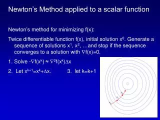
Newton’s Method applied to a scalar function Newton’s method for minimizing f(x):

1. Newton’s Method applied to a scalar function Newton’s method for minimizing f(x): Twice differentiable function f(x), initial solution x0. Generate a sequence of solutions x1, x2, …and stop if the sequence converges to a solution with f(x)=0. Solve -f(xk) ≈ 2f(xk)x Let xk+1=xk+x. 3. let k=k+1

2. Newton’s Method applied to LS Not directly applicable to most nonlinear regression and inverse problems (not equal # of model parameters and data points, no exact solution to G(m)=d). Instead we will use N.M. to minimize a nonlinear LS problem, e.g. fit a vector of n parameters to a data vector d. f(m)=∑ [(G(m)i-di)/i]2 Let fi(m)=(G(m)i-di)/i i=1,2,…,m, F(m)=[f1(m) … fm(m)]T So that f(m)= ∑ fi(m)2 f(m)=∑ fi(m)2] m i=1 m i=1 m i=1

3. NM: Solve -f(mk) ≈ 2f(mk)m LHS:f(mk)j = -∑ 2fi(mk)jF(m)j = -2 J(mk)F(mk) RHS: 2f(mk)m = [2J(m)TJ(m)+Q(m)]m, where Q(m)= 2 ∑ fi(m) fi(m) -2 J(mk)F(mk) = 2 H(m) m m = -H-1 J(mk)F(mk) = -H-1f(mk) (eq. 9.19) H(m)= 2J(m)TJ(m)+Q(m) fi(m)=(G(m)i-di)/i i=1,2,…,m, F(m)=[f1(m) … fm(m)]T

4. Gauss-Newton (GN) method 2f(mk)m = H(m) m = [2J(mk)TJ(mk)+Q(m)]m ignores Q(m)=2∑ fi(m) fi(m) : f(m)≈2J(m)TJ(m), assuming fi(m) will be reasonably small as we approach m*. That is, Solve -f(xk) ≈ 2f(xk)x f(m)j=∑ 2fi(m)jF(m)j, i.e. J(mk)TJ(mk)m=-J(mk)TF(mk) fi(m)=(G(m)i-di)/i i=1,2,…,m, F(m)=[f1(m) … fm(m)]T

5. Newton’s Method applied to LS Levenberg-Marquardt (LM) method uses [J(mk)TJ(mk)+I]m=-J(mk)TF(mk) ->0 : GN ->large, steepest descent (SD) (down-gradient most rapidly). SD provides slow but certain convergence. Which value of  to use? Small values when GN is working well, switch to larger values in problem areas. Start with small value of , then adjust.

6. Statistics of iterative methods Cov(Ad)=A Cov(d) AT (d has multivariate N.D.) Cov(mL2)=(GTG)-1GT Cov(d) G(GTG)-1 Cov(d)=2I: Cov(mL2)=2(GTG)-1 However, we don’t have a linear relationship between data and estimated model parameters for the nonlinear regression, so cannot use these formulas. Instead: F(m*+m)≈F(m*)+J(m*)m Cov(m*)≈(J(m*)TJ(m*))-1 not exact due to linearization, confidence intervals may not be accurate :) ri=G(m*)i-di , i=1 s=[∑ ri2/(m-n)] Cov(m*)=s2(J(m*)TJ(m*))-1 establish confidence intervals, 2

7. Implementation Issues Explicit (analytical) expressions for derivatives Finite difference approximation for derivatives When to stop iterating? f(m)~0 ||mk+1-mk||~0, |f(m)k+1-f(m)k|~0 eqs 9.47-9.49 4. Multistart method to optimize globally

8. Iterative Methods SVD impractical when matrix has 1000’s of rows and columns e.g., 256 x 256 cell tomography model, 100,000 ray paths, < 1% ray hits 50 Gb storage of system matrix, U ~ 80 Gb, V ~ 35 Gb Waste of storage when system matrix is sparse Iterative methods do not store the system matrix Provide approximate solution, rather than exact using Gaussian elimination Definition iterative method: Starting point x0, do steps x1, x2, … Hopefully converge toward right solution x

9. Iterative Methods Kaczmarz’s algorithm: Each of m rows of Gi.m = didefine an n-dimensional hyperplane in Rm Project initial m(0) solution onto hyperplane defined by first row of G Project m(1) solution onto hyperplane defined by second row of G … until projections have been done onto all hyperplanes Start new cycle of projections until converge If Gm=d has a unique solution, Kaczmarz’s algorithm will converge towards this If several solutions, it will converge toward the solution closest to m(0) If m(0)=0, we obtain the minimum length solution If no exact solution, converge fails, bouncing around near approximate solution If hyperplanes are nearly orthogonal, convergence is fast If hyperplanes are nearly parallel, convergence is slow

10. Conjugate Gradients Method Symmetric, positive definite system of equations Ax=b min (x) = min(1/2 xTAx - bTx) • (x) = Ax - b = 0 or Ax = b CG method: construct basis p0, p1, … , pn-1 such that piTApj=0 when i≠j. Such basis is mutually conjugate w/r to A. Only walk once in each direction and minimize x = ∑ipi - maximum of n steps required! () = 1/2 [ ∑ ipi]TA∑ipi - bT [∑ipi] = 1/2 ∑∑ijpiTApj - bT [∑ipi] (summations 0->n-1) n-1 i=0

11. Conjugate Gradients Method piTApj=0 when i≠j. Such basis is mutually conjugate w/r to A. (pi are said to be ‘A orthogonal’) () = 1/2 ∑∑ijpiTApj - bT [∑ipi] = 1/2 ∑ipiTApi - bT [∑ipi] = 1/2 (∑ipiTApi - 2 ibT pi) - n independent terms Thus min () by minimizing ith term ipiTApi - 2 ibT pi ->diff w/r i and set derivative to zero:i = bTpi / piTApi i.e., IF we have mutually conjugate basis, it is easy to minimize ()

12. Conjugate Gradients Method CG constructs sequence of xi, ri=b-Axi, pi Start: x0, r0=b, p0=r0, 0=r0Tr0/p0TAp0 Assume at kth iteration, we have x0, x1, …, xk; r0, r1, …, rk; p0, p1, …, pk; 0, 1, …, k Assume first k+1 basis vectors pi are mutually conjugate to A, first k+1 ri are mutually orthogonal, and riTpj=0 for i ≠j Let xk+1= xk+kpk and rk+1= rk-kApk which updates correctly, since: rk+1 = b - Axk+1 = b - A(xk+kpk) = (b-Axk) - kApk = rk-kApk

13. Conjugate Gradients Method Let xk+1= xk+kpk and rk+1= rk-kApk k+1 = rk+1Trk+1/rkTrk pk+1= rk+1+k+1pk bTpk=rkTrk (eq 6.33-6.38) Now we need proof of the assumptions rk+1 is orthogonal to ri for i≤k (eq 6.39-6.43) rk+1Trk=0 (eq 6.44-6.48) rk+1 is orthogonal to pi for i≤k (eq 6.49-6.54) pk+1TApi = 0 for i≤k (eq 6.55-6.60) i=k: pk+1TApk = 0 ie CG generates mutually conjugate basis

14. Conjugate Gradients Method Thus shown that CG generates a sequence of mutually conjugate basis vectors. In theory, the method will find an exact solution in n iterations. Given positive definite, symmetric system of eqs Ax=b, initial solution x0, let 0=0, p-1=0,r0=b-Ax0, k=0 If k>0, let k = rkTrk/rk-1Trk-1 Let pk= rk+kpk-1 Let k = rkTrk / pkTApk 4. Let xk+1= xk+kpk 5. Let rk+1= rk-kApk 6. Let k=k+1

15. Conjugate Gradients Least Squares Method CG can only be applied to positive definite systems of equations, thus not applicable to general LS problems. Instead, we can apply the CGLS method to min ||Gm-d||2 GTGm=GTd

16. Conjugate Gradients Least Squares Method GTGm=GTd rk = GTd-GTGmk = GT(d-Gmk) = GTsk sk+1=d-Gmk+1=d-G(mk+kpk)=(d-Gmk)-kGpk=sk-kGpk Given a system of eqs Gm=d, k=0, m0=0, p-1=0, 0=0, r0=GTs0. If k>0, let k = rkTrk/[rk-1Trk-1] Let pk= rk+kpk-1 Let k = rkTrk / [Gpk]T[Gpk] 4. Let mk+1= mk+kpk 5. Let sk+1=sk-kGpk 6. Let rk+1= rk-kGpk 7. Let k=k+1; never computing GTG, only Gpk, GTsk+1

17. L1 Regression LS (L2) is strongly affected by outliers If outliers are due to incorrect measurements, the inversion should minimize their effect on the estimated model. Effects of outliers in LS is shown by rapid fall-off of the tails of the Normal Distribution In contrast the Exponential Distribution has a longer tail, implying that the probability of realizing data far from the mean is higher. A few data points several  from <d> is much more probable if drawn from an exponential rather than from a normal distribution. Therefore methods based on exponential distributions are able to handle outliers better than methods based on normal distributions. Such methods are said to be robust.

18. L1 Regression min ∑ [di -(Gm)i]/i = min ||dw-Gwm||1 thus more robust to outliers because error is not squared Example: repeating measurement m times: [1 1 … 1]T m =[d1 d2 … dm]T mL2 = (GTG)-1GTd = m-1∑ di f(m) = ||d-Gm||1 = ∑ |di-m| Non-differentiable if m=di Convex, so local minima=global minima f’(m) = ∑ sgn(di-m), sgn(x)=+1 if x>0, =-1 if x<0, =0 if x=0 =0 if half is +, half is - <d>est = median, where 1/2 of data is < <d>est, 1/2 > <d>est

19. L1 Regression Finding min ||dw-Gwm||1is not trivial. Several methods available, such as IRLS, solving a series of LS problems converging to a 1-norm: r=d-Gm f(m) = ||d-Gm||1 = ||r||1 = ∑ |ri| non-differentiable if ri=0. At other points: f’(m) = ∂f(m)/∂mk = - ∑ Gi,k sgn(ri) = -∑ Gi,k ri/|ri| f(m) = -GTRr = -GTR(d-Gm) Ri,i=1/|ri| f(m) = -GTR(d-Gm) = 0 GTRGm = GTRd R depends on m, nonlinear system :( IRLS!

20. convolution S(t)=h(t)*f(t) = ∫h(t-k) f(k) dk = ∑ ht-k fk h1 0 0 s1 assuming h(t) and f(t) are of length h2 h1 0 s2 5 and 3, respectively h3 h2 h1 f1 s3 h4 h3 h2 f2 =s4 h5 h4 h3 f3 s5 0 h5 h4 s6 0 0 h5 s7 Here, recursive solution is easy

21. convolution ‘Shaping’ filtering: A*x=D, D ‘desired’ response, A,D known a1 a2 a3 a0 a1 a2 a-1 a0 a1 . The matrix ij is formed by the auto-correlation of at with zero-lag values along the diagonal and auto-correlations of successively higher lags off the diagonal. ij is symmetric of order n a1 a0 a-1 a2 a1 a0 a3 a2 a1 .    

22. convolution ATD becomes . a-1 a-2 a-3 a0 a-1 a-2 a1 a0 a-1 . The matrix cij is formed by the cross-correlation of the elements of A and D. Solution: (ATA)-1ATD = -1c . d-1 d0 d1 . . c1 = c0 c-1 .

23. Example Find a filter, 3 elements long, that convolved with (2,1) produced (1,0,0,0): (2,1)*(f1,f2,f3)=(1,0,0,0) a-1 a-2 a-3 a0 a-1 a-2 a1 a0 a-1 . The matrix cij is formed by the cross-correlation of the elements of A and D. Solution: (ATA)-1ATD = -1c c1 = c0 c-1 . d-1 d0 d1 .