Shaocai Yu * , Brian Eder* ++ , Robin Dennis* ++ , Shao-hang Chu**, Stephen Schwartz***

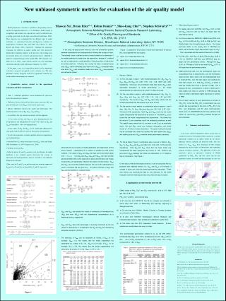
1. New unbiased symmetric metrics for evaluation of the air quality model •  1.   INTRODUCTION • Model performance evaluation is a problem of longstanding concern, and has two important objectives, i.e., (1) determine a model’s degree of acceptability and usefulness for a specific task, and (2) establish that one is getting good results for the right reason (Russell and Dennis, 2000). These objectives are accomplished by two different types of model evaluation, i.e., operational evaluation and diagnostic evaluation (or model physics evaluation) (Fox, 1981; EPA, 1991; Weil et al., 1992; Russell and Dennis, 2000), respectively. Although the operational evaluations for different air quality models have been intensively performed for regulatory purposes in the past years, the resulting array of statistical metrics are so diverse and numerous that it is difficult to judge the overall performance of the models (EPA, 1991; Seigneur et al., 2000; Yu et al., 2003). Some statistical metrics can cause misleading conclusions about the model performance (Seigneur et al., 2000). • In this paper, a new set of quantitative metrics for the operational evaluation is proposed and applied in real evaluation cases. The other quantitative metrics frequently used in the operational evaluation are tested and their shortcomings are examined. • 2. Quantitative metrics related to the operational evaluation and their examinations • Table 1: traditional quantitative metrics,mathematical expressions used in the operational evaluation. • Differences between the model and observations: mean bias (MB) and mean absolute gross error (MAGE) (or root mean square error). • Relative differences between the model and observations: The traditional metrics (such as MNB, MNGE, NMB,and NME) • two problems that may mislead conclusions with this approach: (1) the values of MNB and NMB can grow disproportionately for overpredictions and underpredicitons because both values of MNB and NMB are bounded by –100% for underprediction; (2) the values of MNB and MNGE can be significantly influenced by some points with trivially low values of observations (denomination). • To solve this asymmetric evaluation problem between overpredictions and underpredictions, • fractional bias (FB) and fractional gross error (FGE) (Irwin and Smith, 1984; Kasibhatla et al., 1997; Seigneur et al., 2000). • Problems for FB and FGE: • what the metrics FB and FGE measure is not clear because the model prediction is not evaluated against observation but average of observation and model prediction, which is contradict to the traditional definition of evaluation. • the scales of FB and FGE are not linear and are seriously compressed beyond 1 as FB and FGE are bounded by 2 and +2, respectively. • Table 3 and Figures 3 and 4: • For weekly data from CASTNet, both NMBF (0.03 to 0.08) and NMEF (0.24 to 0.27) for SO42- are lower than the performance criteria. • For 24-hour data from IMPROVE, SEARCH and STN, both NMBF (-0.19 to 0.22) and NMEF (0.42 to 0.46) for SO42- are slightly higher than the performance criteria. The model performed better on the weekly data of CASTNet and better over the eastern region than western region for SO42-. This is consistent with the results of Dennis et al. [1993]. • For PM2.5 NO3-, both NMBF (-0.96 to 0.59) and NMEF (0.80 to 1.70) for SEARCH, CASTNet, and IMPROVE data are larger than the performance criteria. Although the NMBF (0.01) for STN data in 2002 is very small, its NMEF (0.77) is still larger than the performance criteria. • CMAQ performed well over the Northeastern region but overpredicted most of observed NO3- over the mid-Atlantic region by more than a factor of 2 and underpredicted most of observed NO3- over the west region and southeast by more than a factor of 2. Both NMBF and NMEF of winter of 2002 are smaller than those of summer of 1999. This is because the NO3- concentrations in winter of 2002 were 7 times higher than those in summer of 1999 although MB values of winter of 2002 were higher than those of summer of 1999. • One of major reasons for poor performance of model on PM2.5 NO3- is that the PM2.5 NO3- concentrations are very low and are very sensitive to the errors in PM2.5 SO42- and NH4+, and temperature and RH when thermodynamic model (such as ISSORROPIA model here) partitions total nitrate (i.e., aerosol NO3-+gas HNO3) between the gas and aerosol phases. • 4.      Summary and conclusions • A set of new statistical quantitative metrics on the basis of concept of factor has been proposed that can provide a rational operational evaluation of air quality model for the relative difference between modeled and observed results. The new metrics (i.e., NMBF, NMEF) have advantages of both avoiding dominance by the low values of observations and maintaining adequate evaluation symmetry. The application of these new quantitative metrics in operational evaluation of CMAQ performance on PM2.5 SO42- and NO3- shows that the new quantitative metrics are useful and their meanings are also very clear and easy to explain. Shaocai Yu*, Brian Eder*++, Robin Dennis*++, Shao-hang Chu**, Stephen Schwartz*** *Atmospheric Sciences Modeling Division, National Exposure Research Laboratory, ** Office of Air Quality Planning and Standards, U.S. EPA, NC 27711 *** Atmospheric Sciences Division, Brookhaven National Laboratory, Upton, NY 11973 ++Air Resources Laboratory, National Oceanic and Atmospheric Administration, RTP, NC 27711 • Figure 1: a dataset for a real case of model and observation for aerosol NO3- was separated into four regions, • region 1 for model/observation0.5, • region 2 for 0.5model/observation1.0, • region 3 for 1.0<model/observation2.0, • region 4 for 2.0model/observation. • Results in Table 2: • for the only data in region 1 with model/observation0.5, MNB, NMB, FB, NMFB, MNFB and NMBF are –0.82, -0.78, -1.43, -1.28, -36.67, and –3.58, respectively. Obviously, only normalized mean bias factor (NMBF) gives reasonable description of model performance, i.e., the model underpredicted the observations by a factor of 4.58 in this case. • For the only data in region 4 with model/observation>2, MNB, NMB, FB, NMFB, MNFB and NMBF are 4.27, 2.25, 1.12, 1.06, 4.27 and 2.25, respectively. The results of NMBF and NMB reasonably indicate that the model overpredicted the observations by a factor of 3.25. • For the results of each metrics on combination case of regions 1 and 4 data, MNB, NMB, FB, NMFB, MNFB and NMBF are 1.50, 0.06, -0.27, 0.06, -18.02 and 0.06, respectively. Both NMB and NMBF show that the model slightly overpredicted the observations by a factor of 1.06, while FB (-0.27) shows that the model underpredicted the observations. This shows that the value of FB can sometimes result in a misleading conclusion as well. This specific case shows that it is not wise to use FB as an evaluation metric. NME and NMEF: gross error between observations and model results is 1.19 times of mean observation. The good model performance can be concluded only under the condition that both relative bias (NMBF) and relative gross error (NMEF) meet the certain performance standards. • For the all data in Figure 1 (combination case 1+2+3+4 in Table 2), MNB, NMB, FB, NMFB, MNFB and NMBF are 0.96, 0.09, -0.13, 0.09, -10.75 and 0.09, respectively. Both NMB and NMBF show that the mean model only overpredicted the mean observation by a factor of 1.09. However, the gross error (NMGE) between the model and observation is 0.77 times as high as observation. See Figure 1. • On the basis of the above analyses and test, it can be concluded that our proposed new statistical metrics (i.e., NMBF and NMEF) on the basis of concept of factor can show the model performance reasonably. These new metrics use observational data as only reference for the model evaluation and their meanings are also very clear and easy to explain. • 3. Applications of new metrics over the US • CMAQ model on PM2.5 SO42- and NO3- over the US: 6/15 to 7/17, 1999 and 1/8 to 2/18, 2002. • PM2.5 SO42- and NO3- observational data: • at 61 rural sites from IMPROVE. Two 24-hour samples are collected on quartz filters each week, on Wednesday and Saturday, beginning at midnight local time. • at 73 rural sites from CASNet. Weekly (Tuesday to Tuesday) samples are collected on Teflon filters. • at 8 sites from SEARCH (Southeastern Aerosol Research and Characterization project). Daily samples are collected on quartz filters. • at 153 urban sites from STN (Speciated Trends Network). 24-hour samples are usually taken once every six days. • The recommended performance criteria for O3 by US EPA (1991): normalized bias (MNB) 5 to 15%; normalized gross error (MNGE) 30% to 35%. +15% of MNB corresponds to +15% of NMBF while –15% of MNB corresponds to –18% of NMBF. • In this study, we propose new metrics to solve the symmetrical problem between overprediction and underprediction following the concept of factor. Theoretically, factor is defined as ratio of model prediction to observation if the model prediction is higher than the observation, whereas it is defined as ratio of observation to model prediction if the observation is higher than the model prediction. Following this concept, the mean normalized factor bias (MNFB), mean normalized gross factor error (MNGFE), normalized mean bias factor (NMBF) and normalized mean error factor (NMEF) are proposed and defined as follows: • where Mi and Oi are values of model (prediction) and observation at time and/or location i, respectively, N is number of samples (by time and/or location). The values of MNFB, and NMBF are linear and not bounded (range from - to +). Like MNB and MNGE, MNFB and MNGFE can have another general problem when some observation values (denomination) are trivially low and they can significantly influence the values of those metrics. NMBF and NMEF can avoid this problem because the sum of the observations is used to normalize the bias and error,. The above formulas of NMBF and NMEF can be rewritten for case as follows: • NMBF and NMEF are actually the results of summaries of normalized bias (MNB) and error (MNGE) with the observational concentrations as a weighting function, respectively. • NMBF and NMEF have both advantages of avoiding dominance by the low values of observations in normalization like NMB and NME and maintaining adequate evaluation symmetry. • The meanings of NMBF can be interpreted as follows: if NMBF0, for example, NMBF =1.2, this means that the model overpredicts the observation by a factor of 2.2 (i.e., NMBF+1=1.2+1=2.2); if NMBF0, for example, NMBF =-0.2, this means that the model underpredicts the observation by a factor of 1.2 (i.e., NMBF-1=-0.2-1=-1.2). Acknowledgements The authors wish to thank other members at ASMD of EPA for their contributions to the 2002 release version of EPA Models-3/CMAQ during the development and evaluation. This work has been subjected to US Environmental Protection Agency peer review and approved for publication. Mention of trade names or commercial products does not constitute endorsement or recommendation for use. REFERENCES Cox, W.M., Tikvart, J.A., 1990. Atmospheric Environment 24, 2387-2395. Eder, B., Shaocai, Yu, etc., 2003. Atmospheric Environment (in preparation). EPA, 1991. Guideline for regulatory application of the urban airshed model. USEPA Report No. EPA-450/4-91-013. U.S. EPA, Office of Air Quality Planning and Standards, Research Triangle Park, North Carolina. Dennis, R.L., J.N. McHenry, W.R.Barchet, F.S. Binkowski, and D.W. Byun, Atmos. Environ., 26 A(6), 975-997, 1993. Fox, D.G., 1981. Bulletin American Meteorological Society 62, 599-609. Irwin, J., and M. Smith, 1984, Bulletin American Meteorological Society 65, 559-568 Russell, A., and R. Dennis, Atmos. Environ., 34, 2283-2324, 2000. Seigneur, C., et al.,., 2000. Journal of the Air & Waste Management Association 50, 588-599. Weil, J.C., R.I. Sykes, and A. Venkatram, 1992, Journal of Applied Meteorology, 31, 1121-1145. Yu, S.C., Kasibhatla, P.S., Wright, D.L., Schwartz, S.E., McGraw, R., Deng, A., 2003.Journal of Geophysical Research 108(D12), 4353, doi:10.1029/2002JD002890.