Download
1 / 33
330 likes | 349 Vues
This workshop explores temperature trends in Arctic regions across paleoclimates, present, and future scenarios using CMIP5 model outputs. Discussions include intraseasonal, seasonal, and interannual variations, non-Gaussian internal variability, detectability of cooling trends, necessary data length for trend detection, and more.

E N D
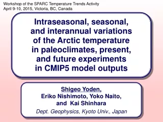
Workshop of the SPARC Temperature Trends Activity April 9-10, 2015, Victoria, BC, Canada Intraseasonal, seasonal, and interannual variations of the Arctic temperature in paleoclimates, present, and future experiments in CMIP5 model outputs Shigeo Yoden, Eriko Nishimoto, Yoko Naito, and Kai Shinhara Dept. Geophysics, Kyoto Univ., Japan
stratosphere troposphere • Non-Gaussian nature of internal interannual variability • Nishizawa and Yoden (2005, JGR ) • “Distribution functions of a spurious trend in a finite length data set with natural variability” in an MCM • normalized pdfs of monthly [T] at the North Pole
Natural variability small in summer (July) large in winter (Feb.) • Detectability of cooling trend with a finite-length data • 96 ensembles of 50-year integration • with external linear trend • - 0.25K/year around 1hPa • Example of cooling trend run • 96 ensembles of 50-year integration • with external linear trend -0.25K/year around 1hPa
Seasonally dependent detectability • How many years do we need to get a statistically significant trend ? • How small trend can we detect in finite length data with a statistical significance ? necessary data length [years] to detect a linear trend of - 0.5K/decade with 90% conf. necessary magnitude of the trend [K/decade] to detect with a 20-year dataset 0.1 pressure [hPa] 0.5 25 10 100 Jan Dec month T(North Pole)
(1979~1997) 1. Introduction • Intraseasonal and interannual variations of polar temperature: largely internal variation in the nonlinear system, such as SSW, vortex intensification, … vs. external forcings such as volcanic eruption, solar cycle, anthropogenic effects, etc. • Seasonal cycle: periodic response to the external solar forcing (revolution of the earth) with large difference between the two poles in dynamically active season (Yoden et al. , 2001)
Polar-night Jet Oscillation (PJO): an important component of intraseasonal variations Kuroda and Kodera (2001) • low-frequency internal variations in polar winter • correspondence to the occurrence of SSW and VI • slow descent of temperature anomaly at the North Pole to the upper troposphere
Motivation: What’s about such intraseasonal, seasonal, and interannual variations in the Arctic temperature in paleoclimates, present or future climate ? • Purpose of this study: Analyses (fundamental statistics, EOF, cluster) of CMIP5 model outputs to make model intercomparison Paleoclimates: • Last Glacial Maximum (LGM) 21,000 BP(before present) • Mid-Holocene (MN) 6,000 BP Present: • Pre Industrial Control (PI) 1,850 AD Future: • Abrupt 4xCO2 (4xCO2)
2. CMIP5 model output data • Seven models • Four experiments
3. Fundamental statistics • Vertical profiles of annual and global mean temperature LGM CO2 = 185 ppm MH 280 ppm 285 ppm PI 1140 ppm 4xCO2 LGM – PI MH – PI 4xCO2 – PI MIROC-ESM MPI-ESM-P MRI-CGCM3 IPSL-CM5A-LR GISS-E2-R CCSM4 CNRM-CM5
Latitude-height sections of seasonal and zonal mean temperature (seven model ensemble-mean) DJF LGM MH PI 4xCO2 JJA LGM MH PI 4xCO2
Latitude-height sections of seasonal and zonal mean temperature difference from PI Control DJF LGM – PI MH – PI 4xCO2 – PI JJA LGM – PI MH – PI 4xCO2 – PI
Latitude-height sections of standard deviations among seven models on seasonal & zonal mean temperature DJF LGM MH PI 4xCO2 JJA LGM MH PI 4xCO2
Month-to-month variations of North Pole temperature for seven models in four experiments LGM MH PI 4xCO2 10 hPa 100 hPa 700 hPa MIROC-ESM MPI-ESM-P MRI-CGCM3 IPSL-CM5A-LR GISS-E2-R CCSM4 CNRM-CM5
Month-to-month variations of the standard deviation (interannual variation) of North Pole temperature for seven models in four experiments LGM MH PI 4xCO2
4. EOF analysis of North Pole temperature • T(925 hPa < p < 10 hPa, t) • 7 models x 4 experiments x 100 years = 2,800 years x 12 months = 33,600 months EOF1 EOF2 (70.2%) (16.6%)
Month-to-month variation of distribution in (PC1, PC2) large amplitude 10 % “extreme” other 90% warm cold events events
Histograms of extreme (top 10% large-amplitude) events cold events warm events cold events phase angle
Time-height composites of extremely warm events for each month Nov (81, 95.3%) Dec (234, 79.1%) Jan (393, 59.9%) Feb (553, 53.2%) Mar (515, 54.7%) Apr (151, 44.8%)
Time-height composites of extremely cold events for each month Nov (4, 4.7%) Dec (62, 20.9%) Jan (263, 40.1%) Feb (486, 46.8%) Mar (427, 45.3%) Apr (186, 55.2%)
Month-to-month variations of extremely warm events andcold events (33,600 months x 10% = 3,360 month)
Month-to-month variations of extremely warm events andcold events for LGM, MH, PI, and 4xCO2
Month-to-month variations of extremely warm events and cold events for seven models • High top: MIROC, MPI, MRI • Middle: IPSL, GISS • Low top: CCSM4, CNRM
5. Cluster analysis of North Pole temperature • In EOF analysis, each month is treated independently • Time evolution of (PC1,PC2) for 5 months (D,J,F,M,A) in 7 models x 100 years = 700 years for 4 experiments Distribution of distance Hierarchical Tree Plot number of clusters
Distribution of distancefor LGM, MH, PI, and 4xCO2 LGM MH 4 3 PI 4xCO2 3 4 number of clusters number of clusters
Time-height sections for each cluster in 4 experiments LGM MH PI 4xCO2 warm1(85) warm1(161) warm1(262) warm1(149) warm2(112) warm2(201) warm2(322) warm2(170) warm3(317) cold2(284) cold1(179) cold1(331) cold1(109) cold1(90)
Number of members in each cluster LGM MH PI 4xCO2
Number of members in each cluster divided into each model 1: MIROC 2: MPI 3: MRI 4: IPSL 5: GISS 6: CCSM4 7: CNRM
Time evolution of (PC1,PC2) for 5 months (D,J,F,M,A) in 4 exp. x 100 years = 400 years for 7 models • Distribution of distancefor seven models number of clusters
Number of members in each cluster MIROC MPI MRI IPSL GISS CCSM4 CNRM
Number of members in each cluster divided into each experiment, LGM, MH, PI, and 4xCO2
6. Summary • Intraseasonal, seasonal, and interannual variations in the Arctic temperature are described for four experiments of paleoclimates, present and future climate in CMIP5 model outputs. • Fundamental statistical analysis shows large sensitivity of climatology and variations in dynamically active season, particularly in low top models. • EOF analysis extracts PJO-like variations as extremely warm events and cold events. • Extreme events are more frequent in high-top models than in low-top models. • Cluster analysis can determine intraseasonal evolution of PJO-like oscillation (warm and cold), but we need further experience for better use of it.
Thank you !! 熱帯域の雲 (2007/07/30)