Download
1 / 20
200 likes | 363 Vues
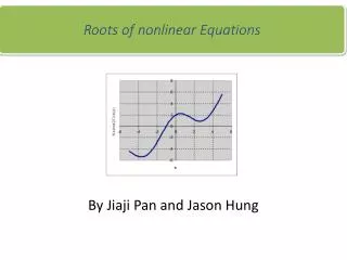
Roots of nonlinear Equations. By Jiaji Pan and Jason Hung. Root for Polynomials. Transfer function of a system Zeros : Poles :. Newton’s method. f(x) given function while and k < N compute , k = k + 1 End Root = . Value of Polynomial . Let

E N D
Roots of nonlinear Equations By Jiaji Pan and Jason Hung
Root for Polynomials Transfer function of a system Zeros: Poles:
Newton’s method f(x) given function while and k < N compute , k = k + 1 End Root =
Value of Polynomial Let Rewrite this polynomial with a given z Where = Then at x = z
Obtained the coefficients of and Comparing the coefficient = = for k = n-1,n-2,…0 The coefficients are computed recursively by knowing (the coefficients of ) Then the value of at a given value z is found ----
Value of Polynomial From rewrite the polynomial with z: Where = =
Obtained the coefficients of and Comparing the coefficient = = for k = n-2,n-3,…0 are computed by knowing (the coefficients of ) Then the value ofat a given z is found ----
Combine Horner’s Method with Newton Method When we do the newton method iteration When f(x) = Now with the Horner’s method.
Algorithm Given: The coefficients of polynomial: initial guess , tolerance, iteration index k = 0,j = 0 do { 1. z = , , 2.compute b for j = n-1,n-2,…,1 = = end 3. = 4. } While | > tolerance
Advantage of this method More efficient additions: 2n vs 2n in newton raphson multiplications : 2n − 2 vs in newton raphson :Do not require to find the derivative of polynomial
Solving for Complex Roots • Note that none of the methods: the Newton, the Secant, the Fixed Point iteration Methods, etc. cannot produce an approximation of a complex root starting from real approximations. • Muller’s Method
Muller’s Method: Steps • Approximate x2 from x0 and x1 • Approximation of x2 is computed as the x-intercept of the secant line passing through (x0,f(x0)) and (x1,f(fx1)) • Approximating x3 from x2, x0 and x1 • Having (x0,f(x0)), (x1,f(x1)) and (x2,f(x2)) at hand, next approximation x3 is computed as the x-intercept of the parabola passing through these three points.
Muller’s Method: Steps • Computer x4 and successive approximations. (ie. xnis approximated using xn-1, xn-2, and xn-3)
Muller’s Method: Math • Let the equation of the parabola P be: P(x) = a(x-x2)2+b(x-x2)+c • Since P(x) passes through (x0,f(x0)), (x1,f(x1)) and (x2,f(x2)), we have: P(x0) = f(x0) = a(x0 – x2)2 + b(x0 – x2) + c P(x1) = f(x1) = a(x1 – x2)2 + b(x1 – x2) + c P(x2) = f(x2) = c
Muller’s Method: Math • Knowing c = f(x2), we can now obtain a and b by solving the first two equations: • From there we can obtain x3 by solving P(x3) = 0. P(x3) = a(x3 – x2)2 + b(x3 – x2) + c = 0
Muller’s Method: Math • To solve for xn-xn-1: • Solving for x3:
Muller’s Method: Example • Given equation: f(x) = x3-2x2-5 • Starting guesses: • x0= -1 • x1 = 0 • x2 = 1
Muller’s Method: Example • Solutions: x = -0.345323724017634 +/- 1.318726779571698i x = 2.690647448028386 • Verify: f(x) = (x+0.34532+1.3187i)*(x+0.34532-1.3187i)*(x- 2.6906) = x3-1.99996x2-0.0000203916x+i(4.4E-16)-4.99971 = x3-2x2-5