Download
1 / 49
490 likes | 586 Vues
Discover the widespread occurrence of magnetism from the scale of galaxies to nanoscale particles in this comprehensive guide to nanomagnetism principles and applications. Learn about magnetic nanoparticles in rocks, magnetotactic bacteria, and the magnetic field of Earth, among other fascinating phenomena. Gain insights into important magnetism concepts, such as the atomic origin of magnetic moments and the behaviors of diamagnetism and paramagnetism. This resource is a valuable read for those interested in the intricate world of magnetism in nanomaterials.

E N D
Magnetism in Nanomaterials Advanced Reading Principles of Nanomagnetism A.P. Guimarães Springer-Verlag, Berlin, 2009.
Introduction to Magnetism Magnetism is virtually universal. • Coherent magnetic fields have been found at the scale of the galaxies and cluster of galaxies. (1-3 G) • Earth's magnetic field has a strength of about 1 G and reverses itself with an average period of about 2105 years. • Magnetic nanoparticles are found in some rocks and can be used to determine the earth's magnetic field (strength and direction) in the past. • Magnetotactic bacteria have nanometer-sized magnets, which they use for alignment with the earth's magnetic field. • Many birds (e.g. the homing pigeon) and other living creatures have clusters of nanoparticles (~2-4 nm in the pigeon) in their beak area, which helps them with their homing ability. • Highest continuous magnetic field obtained is about 45 T (45104G). • Mega-Gauss have been obtained in Femto-seconds. • Magnetars: 1011 T. (Earth is 1000 larger than a typical neutron star).
If a loop of area A is carrying a current I, the intrinsic intensity of the magnetic field is given by the magnetic moment vector (m or ) directed from the north pole to the south pole; such that the magnitude of m is given by: m = IA(units: [Am2]). • The magnetic moment is the measure of the strength of the magnet and is the ability to produce (and be affected by) a magnetic field. Important quantities in magnetism
Atomic origin of magnetic moments This is classical way of looking at a quantum effect !
From magnetism of the fundamental components to magnetism of devices
Diamagnetism • This is a property of all materials in response to an applied magnetic field and hence there is no requirement for the atoms to have net magnetic moments. • This is a weak negative magnetic effect ( ~ 105) and hence may be masked by the presence of stronger effects like ferromagnetism (even though it is still present). • A simplified understanding of the diamagnetic effect (in a more classical way!) is based on Lenz's law applied at the atomic scale. Lenz's law states that change in magnetic field will induce a current in a loop of electrical conductor, which will tend to oppose the applied magnetic field. As the electron velocity is a function of the energy of the electronic states, the diamagnetic susceptibility is essentially independent of temperature. A diamagnet tends to exclude lines of force from the material. • A superconductor (under some conditions) is a perfect diamagnet and it excludes all magnetic lines of force. • Closed shell electronic configuration leads to a net zero magnetic moment (spin and orbital moments are oriented to cancel out each other). Monoatomic noble gases (e.g. He, Ne, Ar, Kr etc.) are diamagnetic. In polyatomic gases (e.g. H2, N2 etc.), the formation of the molecule leads to a closed electronic shell configuration, thus making these gases diamagnetic. Many ionically bonded (e.g. NaCl, MgO, etc.) and covalently bonded (C-diamond, Ge, Si) materials also lead to a closed shell configuration, thus making diamagnetism as the predominant magnetic effect. Most organic compounds (involving other types of bonds as well) are diamagnetic.
A simplified understanding of diamagnetism based on Lenz's law: (a) electrons paired in the same orbital moving with a velocity 'v' canceling each others magnetic moments (m), (b) effect of an increasing magnetic field (B) on the magnetic moments. m1 increases and m2 decreases, so that the net magnetic moment opposes the field B. The M-H plot for a diamagnetic substance
Paramagnetism • There are two distinct types of paramagnetism: (i) that arising when the atom/molecule has a net a magnetic moment, (ii) that come from band structure (Pauli spin or weak spin paramagnetism). • If the net magnetic moments (within the atom/molecule) do not cancel out then the material is paramagnetic. Oxygen for example has a net magnetic moment = 2.85 B per molecule. A point to be noted here is that even if there are many electrons in the atom; most of the moments cancel out, leaving a resultant of a few Bohr magnetons. In the absence of an external field these magnetic moments point in random directions and the magnetization of the specimen is zero. When a field is applied two factors come into picture:(i) the aligning force of the magnetic field (we have already seen what this alignment means!)(ii) the disordering tendency of temperature. • The combined effect of these two factors is that only partial alignment of the magnetic moments is possible and the susceptibility of paramagnetic materials has a small value. For example Oxygen has a m(20C) = 1.36 106 m3/Kg.
Two types of paramagnets can be differentiated: (i) those which are always paramagnetic with no other details to be considered and (ii) those which are ferromagnetic, ferrimagnetic or anti-ferromagnetic (and become paramagnetic on heating) these will have non-zero value for '' in the Curie-Weiss law (as considered below). • Effect of Temperature Any magnetic alignment (which is an ordering phenomenon) is always fighting against the disordering effect of temperature. While mass susceptibility (m) is independent of temperature for a diamagnet, for a general paramagnet it follows the Curie-Weiss law ( ~ TC):Where m is the mass susceptibility [m3/Kg], C is the Curie constant and is in units of temperature and is a measure of the interaction of the atomic magnetic moments (usually thought of as an internal 'molecular/atomic field'- the concept of exchange integral, which we will deal with in the context of ferromagnetism, is the quantum mechanical equivalent of this). Actually, 'molecular field' is a 'force/torque' tending to align adjacent atomic moments. It's typical value is ~ 109 A/m and is much stronger than any continuous field produced in a lab.
If there is no interaction between the atomic magnetic moments; then = 0 and the Curie-Weiss law reduces to the Curie law (e.g. for O2). The variation of the susceptibility for these kinds of behaviour is shown in . '' can be positive (usually with small value) or negative. Negative values of '' imply that the molecular/atomic field is opposing the externally imposed field and thus decreasing the susceptibility of the material. In reality the Curie temperature may not be sharp and further aspects come into the picture which we shall not consider here.
Ferromagnetism (FM) • Ferromagnetism, Antiferromagnetism and Ferrimagnetism involve no new types of magnetic moments; but involve the way the magnetic moments are coupled (arranged). • Two important ways of understanding ferromagnetism in metals are: (as listed in the introduction to the magnetic properties): (i) assuming that moments are localized to atoms, (ii) using the band structure of metals (giving rise to itinerant electrons). The former is conceptually easier and has been assumed in the 'molecular field theory' and the Heisenberg's approach. It should be noted right at the outset that even in metals (e.g. Fe), most of the electrons behave as if they are 'localized' and the number of itinerant electrons could be a small number. In Fe there are 8 valence electrons which occupy the (3d + 4s) bands. Out of these 8 electrons only ~0.95 in the 4s band are 'truly' free/itinerant and remaining ~7.05 are occupy the 'localized' 3d band. In Ni the corresponding quantities are: (3d + 4s) = 10, free 4s0.6, localized 3d9.4.
Band Theory to Understand Ferromagnetism • As mentioned before a correct theory of magnetism in metals has to involve bands as the electrons are not localized to atoms. However, as noted before, most of the electrons (especially in 3d metals which are elemental magnets) are rather localized and the 'free' electrons (4s) do not contribute to the ferromagnetic behaviour. Truly speaking the 3d electrons in transition metals are neither fully localized nor fully free.Band theory is able to explain the non-integral values of magnetic moment per atom; though, the values may often not match exactly. • The density of states varies in a complicated manner. • In Fe the 3d electrons are all not fully localized and about 5-8% have some itinerant character and these electrons mediate the exchange coupling between the localized moments. Using the observed magnetic moment per atom (H) of Fe to be 2.2B the up-spin and down-spin occupancy can be calculated as: ,
The above discussions can be summarized as a few thumb-rules for existence of ferromagnetism in metals: (i) the bands giving rise to magnetism must have vacant levels (e.g. 3d bands in Fe, Co, Ni) for unpaired electrons to be promoted to; (ii) close to the Fermi level the density of states should be high– this ensures that when electrons are promoted to the unfilled higher energy levels the energy cost is small (high density of states implies a smaller spacing in energy); (iii) assuming direct exchange, the interatomic distance should be correct for exchange forces to be operative (leading to parallel alignment).
Effect of External Magnetic Field • Important parameters marked on the curve are Saturation Induction (Bs), Retentivity (Br) and Coercivity (Hc). The coercivity in an M-H plot is called 'Intrinsic Coercivity' (Mic or Mci). Saturation magnetization is a structure insensitive property while coercivity is a structure sensitive property (coercivity of nanoparticles is different from that of bulk materials). • In 'permanent magnet' applications a high coercivity value is usually desired. Another quantity marked in the figure is the permeability (maximum and initial). Permeability (measured as the slope of the line from the origin to a point) is also a structure sensitive property. The field required to bring a ferromagnet to saturation (Ms) at room temperature is small (~80 kA/m); but, further increase in magnetization would require much stronger fields and this effect is called 'forced magnetization'. B = 0 (H + M)
Alignment of domains leading to magnetization of the sample • Preferential alignment of domains can be brought about by an external magnetic field. During magnetization the domains oriented favourably (along the field direction), grow at the expense of the unfavourably oriented domains. This can occur by: (i) domain wall motion (smooth or jerky) and (ii) by rotation of the magnetization of the domains. The external magnetic field tends to align the misoriented spins in the domain wall- leading to its displacement. These processes can occur simultaneously as the field increases. Rotation of spin is opposed by the increase in anisotropy energy (magnetocrystalline, shape, stress). During rotation all spins need not be parallel to one another and the actual picture may be a little complicated.
Effect of Temperature • Spatially correlated collective quantized modes lead to demagnetization (called spin waves (or magnons)). • Ferromagnet becomes paramagnet above Curie temperature (Tc). At Tcsusceptibility becomes infinite. Even beyond Tc there are local clusters ('spin clusters') of aligned magnetic moments. • Maximum magnetization is obtained when all the moments have parallel orientation– let this state correspond to a magnetization M0 (or 0). • It is expected that a plot of s/0 versus T/Tc will approximately lie on one another for different materials. Demagnetization curve for a ferromagnet.
Domain structure and the Magnetization Process • The magnetic structure of a ferromagnetic material consists of domains → to reduce magnetostatic energy. • Domains are separated by domain walls. Broadly two types of domain walls can be differentiated: Bloch walls and Néel walls. Other types of domain walls like cross-tie walls and more complicated configurations are also possible. As shown in in Bloch walls the spin vectors rotate out of plane in the domain wall (while in Néel walls they rotate in plane). Néel walls are seen in thin films (they are usually observed in thin films ~40 nm thick). Usually the domain wall thickness is few hundred atomic diameters (i.e. it is rather diffuse). Hence, the domain wall by itself is a nanostructure. Actual domain structure more complicated than this
The domain wall represents a region of high energy as the spin vectors are not in the directions of easy magnetization. Hence thicker walls represent higher energy and in materials with high magnetocrystalline anisotropy energy (EA; e.g rare-earth metals), the domain walls are thin (~10 atomic diameters). • Other sources of anisotropy are those due to shape of the particle and due to residual (or applied) stresses. A competition between the magnetostatic energy and the magnetocrystalline anisotropy energy, essentially decides the domain size/shape. • The word 'essentially' has been used as other factors like magnetoelastic energy (EMagnetoelastic = EME) due to magnetostriction (change in dimension due to a magnetic field) also contribute to the overall energy. • The total energy (ETotal) can be written as a sum of four terms: Wherein, EExternal corresponds to the energy of total magnetic moment in the external magnetic field.
Magnetism in Nanomaterials Magnetic nanostructures in bulk materials Even in bulk magnetic materials some structures can be in the nanoscale: • Domain walls in a ferromagnet (~60nm for Fe). • Some domains (especially those in the vicinity of the surface or grain boundaries), could themselves be nanosized. • Spin clusters above paramagnetic Curie temperature (p) could be nano-sized. When we go from bulk to ‘nano’ only the structure sensitive magnetic properties (like coercivity) is expected to change significantly. Some of the possibilities when we go from bulk to nano are: • Ferromagnetic particles becoming single domain • Superparamagnetism in small ferromagnetic particles (i.e. particles which are ferromagnetic in bulk) • Giant Magnetoresistance effect in hybrids (layered structures) • Antiferromagnetic particles (in bulk) behaving like ferromagnets etc.
Dependence of magnetic moment on the dimensionality of the system • There is an increase in magnetic moment/atom as we decrease the dimensionality of the system. • This is indicative of fundamental differences in magnetic behaviour between nano-structures and bulk materials. • This effect is all the more noteworthy as surface spins are usually not ordered along the same directions as the spins in the interior of the material (thus we expect nanocrystals with more surface to have less B/atom than bulk materials- purely based on surface effect). Increasing magnetic moment/atom Fe can have a maximum possible moment of 6B/atom (3B orbital + 3B spin) this implies that in 0D nanocrystals very little of the orbital magnetic moment is quenched
Superparamagnetism • As the size of a particle is reduced the whole particle becomes a single domain below a critical size. • This aspect can be understood in two distinct ways: i) a particle smaller than the domain wall thickness cannot sustain a domain wall (noting that domain wall thickness may not be constant with size), ii) the magnetostatic energy increases as r3('r' being the radius of the particle) and the domain wall energy is a function of r2 there must be a critical radius (rc) below which domain walls are not stable.(in reality the calculation is complicated by other factors). • The general trend is:
2-3 orders of magnitude M vs H/T curve for a superparamagnetic material
Comparison between paramagnetism and superparamagnetism • Magnetization of oxygen (() = 2.85 B per molecule (= 2.64 1023 Am2/molecule); Number of oxygen molecules = (6.023 1023)/0.032 per kg, Magnetic field applied = 20106 A/m; m (20C) = 1.36 106 m3/Kg). • What is the magnetizing effect of the strong field? • If all the magnetic moments of all the molecules are aligned the magnetic moment obtained = ((6.023 1023)/0.032)(2.64 1023) = 497 Am2/kg.The actual magnetization in the presence of the field () = m H = (1.36106)(20106) = 27.2 Am2/kg.Percentage of possible magnetization = (27.2/497)100 ~ 5.5%Thus, even strong fields are very poor in aligning the magnetic moments of paramagnetic materials. • What is the magnetization of Fe nanoparticle (d = 15nm) when saturated (Given: eff(Fe) = 2.2 B; a(Fe) = 2.87 Å). Volume of the particle = 4(15/2)3/3 = 1767 nm3 = 1.767106 Å3 Volume per atom in BCC Fe = (2.87)3/2 = 11.82 Å3 (the factor 2 in the denominator is due to 2 atoms/cell in BCC). Number of atoms of Fe in the particle = 149492 atoms Magnetic moment of the particle under saturation = 328883 B (Bohr magnetons) Check
Magnetism of Clusters • Like other properties of clusters, magnetic properties of clusters can change with the addition (or removal) of an atom. Clusters considered here have few to a thousand of atoms typically (extending upto about 5 nm). • Important factors which determine the magnetic behaviour of clusters are: (i) atomic structure, (ii) nearest neighbours distance, (iii) purity and defect structure of the cluster.
Ferromagnetic clusters • In small clusters (with less than 20 atoms) there are large oscillations in the magnetic moment of the cluster (calculated as magnetic moment per atom). • For more than 600 atoms in the cluster 'bulk-like' behaviour emerges (i.e. with increasing number of atoms the oscillations die down and bulk behaviour emerges). • Fe can have a maximum possible moment of 6B/atom (3B orbital + 3B spin). Fe12cluster has a moment of 5.4B/atom practically very little of the orbital moment is quenched in the cluster. Fe13however has a moment of only 2.44B. Ni13cluster has an abnormally low moment as well and this is attributed to the icosahedral structure of the cluster (which is densely packed). With larger and larger cluster size the orbital contribution seems to be low; but, there is still an enhancement of the magnetic moment over the bulk value. Thus structure and packing seem to play an important role in the net magnetic moment obtained.
Antiferromagnetic clusters • In antiferromagnetic materials we do not expect any net magnetic moment in the bulk. However, there is a possibility that in small clusters 'up' spins do not cancel out the 'down' spins (leading to a net magnetic moment) these are anti-ferromagnets behaving as ferromagnets! • Magnetic 'frustration' is also a possibility. (frustration the spin on a given atom does not 'know' which way to point). • Small clusters of Cr (one of the few metals which are antiferromagnetic- spin density wave AFM) have an interesting rich set of possibilities (along with allied complications!). A plot of magnetic moment per atom oscillates with size (as in the case of ferromagnetic clusters). A given cluster size (e.g. Cr9) is expected to exist in multiple magnetization states (in the case of Cr9 magnetization can be small (~0.65 B/atom) or as high as ~1.8 B/atom [1]). In addition to the 'multiple magnetization states' there is a possibility of co-existence structural isomers. • Mn clusters show some similarities with ferromagnetic Fe clusters with regard to cluster size dependence (with more than 10 atoms) [2]. Compact Mn13(icosahedral) and Mn19 (double-icosahedral) clusters have very low magnetic moment as compared to neighbouring clusters. Mn15has the highest moment of 1.5 B/atom [2]. [1] L. A. Bloomfield, J. Deng, H. Zhang, and J. W. Emmert, in “Clusters and Nanostructure Interfaces” (P. Jena, S. N. Khanna, and B. K. Rao, Eds.), p. 213. World Scientific, Singapore, 2000. [2] M. B. Knickelbein, Phys. Rev. Lett. 86, 5255 (2001).
Mn M. B. Knickelbein, Phys. Rev. Lett. 86, 5255 (2001).
Experimental production of clusters • A gas phase supersaturated metal vapour is ejected into flowing inert gas (which is cooled). • The metal vapour is produced by: (i) thermal evaporation, (ii) laser ablation, (iii) sputtering, etc. • Most mass separators require the clusters to be charged (the clusters need to be ionized if they are not charged). Examples of mass filters include: Radio Frequency Quadrupole filter, Wien filter, Time-of-flight mass spectrometer, Pulsed field mass selector, etc. • At the end of separation we can get a narrow distribution of masses of particles (in small clusters we can even get a precise number of atoms in a cluster). Example of a metal vapour production method
Measurement of magnetic moment of clusters • The experimental results presented for free clusters [Fe (ferromagnetic clusters) and Cr and Mn (antiferromagnetic clusters)] are typically measured using a setup, which is based on the Stern-Gerlach experiment (that detected electron spin) which is typically coupled with pulsed laser vaporization technique (details in next slide). • A collimated cluster beam is guided into a magnetic field gradient (dB/dz). The field gradient will deflect a cluster with magnetic moment by a distance ‘d’ given by the equation as below (L length of the magnet, D distance from the end of the magnet to the detector, M cluster mass, vx entrance velocity). • For clusters deposited on surfaces other techniques of measurement exist such as: X-Ray Magnetic Circular Dichroism, Dichroism in Photoelectron Spectroscopy, Surface Magneto-Optical Kerr Effect, UHV Vibrating Sample Magnetometry, etc. • For embedded clusters techniques like: Micro-SQUID Measurements, Micro-Hall Probes, etc. can be used to measure the magnetic moments.
Experimental setup for the measurement of magnetic moments Metal clusters are produced by pulsed laser vaporization of a target material into a jet of helium gas Cluster+gas mixture undergoes supersonic expansion on entering vacuum Mass dependent deflection measured perpendicular to the beam in a TOFMS Magnetic deflection of collimated beam Beam is collimated Ionization by Laser
Issues regarding the measurement of magnetic properties of nanomaterials • The measurement of magnetic properties in clusters and nanostructures is needless to say challenging, as compared to their bulk counterparts. • In clusters as the magnetic moment is a sensitive function of the number of atoms in the cluster- the number of atoms have to be known precisely. • Coagulation or contamination of clusters/nanocrystals- either during production or during measurements has to be avoided. Surface oxidation can also severely alter the magnetic properties (e.g. Co-CoO system to be considered). • Temperature plays a key role in the magnetic behaviour of nanoscale systems and hence temperature has to be precisely controlled. • The spin alignment in nanoscale systems (to be considered in coming slides) could be very different from their bulk counterparts and hence models with which experimental results are compared have to take into account the precise geometry of the system and surface effects. • In the case of particles on a substrate or embedded magnetic nanoparticles, the role of the interface and the substrate could be pronounced (i.e. deducing the properties of the free-standing nanoparticles from those measured could be difficult).
Magnetism in thin films, hybrids Illustrative examples Ni Cu (100) • 2D versus 3D behaviourIn the case of Ni films on Cu(100) substrates, when the thickness of the Ni film is greater than 7 monolayers (ML) the systems behaves as a 3D Heisenberg ferromagnet and below 7ML it behaves like a 2D system [1]. In the 2D system all the spins are in the plane, while in the 3D system out of plane spin orientation is also observed. • Curie Temperature of thin filmsIn the case of Fe(110) films (1-3 monolayers) grown epitaxially on Ag(111) substrates the Curie temperature reduces from bulk values to ~100K (~10% of the bulk value) for ~1.5 monolayer films [2]. (Thermal disordering effects are becoming prominent). Fe(110) Ag (111) [1] F. Huang, M. T. Kief, G. J.Mankey, and R. F.Willis, Phys. Rev. B 49 (1994) 3962 [2] Z.Q. Qin, J. Pearson, and S. D. Bader, Phys. Rev. Lett. 67,1646 (1991).
Magnetism of Hybrids: Giant Magnetoresistance (GMR) • As compared to normal (conventional) magnetoresistance, where the change in resistance due to a magnetic field is ~5%; in GMR the change could be of the order of about 80% (or more). weak RKKY type coupling
Carrying forward the concept of GMR sandwich structures, a spin valve (GMR) has been devised. In a 'spin valve', the two ferromagnetic layers have different coercivities and can be switched on at difference field strengths. • An extension of spin valves is obtained by replacing the non-ferromagnetic layer with a thin insulating (tunnel) barrier. This can give rise to an effect known as the Tunnel Magneto-resistance (TMR); wherein, larger impedance, which can be matched to the circuit impedance, is obtained. In TMR, spins travelling perpendicular to the layers, tunnels through the insulating layer and hence the name of the effect. • Applications of TMR effect include: hard drives (with high areal densities), Magnetoresistive Random Access Memory (MRAM), etc. It also forms a fundamental unit in spin electronics with applications such as reprogrammable magnetic logic devices.
Magnetism of Hybrids: Exchange anisotropy • Due to exchange coupling of spins across an interface between a ferromagnetic phase and an antiferromagnetic phase, there is a preferred direction (anisotropy) for the field, which leads to a shift in the hysteresis (M-H) loop. [E.g. Co particles (ferromagnetic) covered with CoO (antiferromagnetic with large crystal anisotropy)]. • Steps involved in creating exchange anisotropy:• Have a single domain FM particle (say Co) in contact with a AFM layer (CoO)• Apply a field above the Néel temperature of the AFM phase to saturate the FM phase• Cool the system below the Néel temperature of the AFM phase to introduce a preferential alignment of spins across the interface (in the AFM phase). The spins in the FM phase will maintain their orientation even after the field is removed.• Construct the usual M-H loop • If the field is removed the spins in the FM phase will flip to the field-cooled orientation, due to the influence of the AFM phase. As the field direction is reversed, the spins across the interface in the AFM (with large crystal anisotropy) oppose the reversal of spins in the FM phase. Hence, the exchange coupling leads to large coercivity value.
Nanodiscs Special spin arrangements with no bulk counterparts • Nanodiscs can exist in vortex spin state. 15 nm thick permalloy discs show the vortex state when the diameter of the disc is above 100 nm. The spin arrangement consists of concentric arrangement of spins on the outside (in the plane of the disc) and with out of plane component towards the centre of the disc. The core radius (wherein the spins are out of plane) is of the order of the exchange length (lExchange, which is about 5 nm for permalloy). Other non-equilibrium configurations of spin may also be observed in nanodiscs (e.g. antivortex, double vortex states). Exchange length (lex) is the characteristic length scale of a magnetic material, below which exchange is dominant over magnetostatic effects.
Nanorings • In nanorings there is no 'core based on spin structure'. As shown in part from the votex state the nanorings may have onion and twisted states of magnetization (which are realized in different parts of the hysteresis loop).