Download
1 / 18
190 likes | 533 Vues
7.2 Means and variances of Random Variables (weighted average). Mean of a sample is X bar, Mean of a probability distribution is μ. Example.

E N D
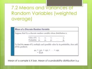
7.2 Means and variances of Random Variables (weighted average) Mean of a sample is X bar, Mean of a probability distribution is μ
Example • Lottery: You choose a 3 digit number. If the lottery shows your same number you win $500. Since there are 1000 possible 3 digit numbers, you have a 1/1000 chance of winning. • What is your average payoff from many tickets? • $500(.001) + $0(.999) = $.50 • How would this differ if you paid 1$ for your ticket?
Mean of a continuous random variable • The point at which the area under the density curve would balance if it were made out of solid material (center if symmetrical). • Mean of skewed density curve requires math outside this course!
Variance of a random Variable • Variance of a random variable X notated as σ2x(different from variance of a sample which is notated as s2).
Example- Linda sells cars We can find the mean and variance of X with a table (or with our calculator! enter X in L1, P in L2, do 1-var stat L1, L2!)
Law of Large Numbers • If we want to estimate the mean height μ of all American women between age 18-24. To estimate μ we take a SRS of F18-24 and use the sample mean X bar to estimate the unknown population mean. • If we repeat this, and choose another sample, the mean height will likely differ, but the more times we repeat this- drawing a sample and recording the mean- we expect that the average of the mean heights of all our samples will get very close to the true μ
The behavior of X bar is just like the behavior of expected probabilities! Example: Suppose the true μ for women’s heights was 64.5 inches with a standard deviation of 2.5 inches. If I continuously repeat drawing a sample of women from this population and recording their average height. After each recording, I write down the average of my mean sample heights. The more times I do this, the closer my overall average gets to 64.5
Casinos, Insurance companies, and law of large numbers • Gamblers may win or lose, but the casino will win in the long run because the law of large numbers says what the average outcome of many thousands of bets will be • This is the same concept when insurance companies decide what to charge or how many beef patties McD’s should make per day
Law of Small numbers • Rules of probability and law of large numbers describe the regular behavior of chance phenomena in the LONG run, but Psychologists have discovered that our intuitive understanding of randomness is quite different from the true laws of chance. • We expect that even short sequences of random events will show the kind of average behavior that in fact only appears in the long run. • Ex: Write down a sequence of heads and tails that you think imitates 10 tosses of a balanced coin. What was the longest run of consecutive heads or tails in your tosses? • Most people don’t write a run of more than 2 consecutive heads or tails. Longer runs don’t seem “random” to us. • In fact, the probability of a run of 3 or more consecutive heads or tails in 10 tosses is greater than .5078! • Seeing a run of 3 or more may cause us to incorrectly conclude that we have a biased coin. • Some gamblers follow “hot-hand” theory…silly!
How large is large? • The law doesn’t say how many trials are needed to guarantee a mean outcome close to μ. • That depends on the variability of the outcomes. • The more variable the outcomes, the more trials are needed to ensure that the mean outcome X bar is close to the distribution mean μ • Casinos understand this: the outcomes of games of chance are variable enough to hold the interest of gamblers. Only the casino plays often enough to rely on the law of large numbers. Gamblers get entertainment, Casino has a business!
Rules for means Review: How can we tell if something is a legitimate probability distribution?
Example (Linda cars) Let X be the number of cars Linda sells and Y the number of trucks and SUV’s. μx = (0)(.3) + (1)(.4) + (2)(.2) + (3)(.1) = 1.1 cars μy = (0)(.4) + (1)(.5) + (2)(.1) = .7 trucks and SUV’s
At her commission rate of 25% of gross profit on each vehicle she sells, Linda expects to earn $350 on each car and $400 on each truck/SUV sold. • her earnings are Z = 350X + 400Y • What are her average (expected) earnings? Combing rules 1 and 2, her mean earnings are • μz = 350 μx + 400 μy = 350x1.1 + 400x .7 = $665 That’s her best estimate of her earnings for the day.
Rules for Variances • For this course we only need to deal with variances of 2 variables that are independent. This is an ASSUMPTION when we do these problems (always ask yourself if the assumption of independence seems reasonable). • RULE 1: Multiplying X by a constant multiplies the SD by that constant (and thus the variance by the square of that constant) • RULE 2: If X and Y are independent σ2x+Y = σx2 + σy2 and σ2x-y = σx2 + σy2 (they’re the same b/c variance affected by the square of the change so doesn’t matter if neg or pos) • The difference X – Y is more variable than either X or Y alone because variations in both X and Y contribute to variation in their difference.
Example: Winning lottery (review) • The payoff X of a $1 ticket (do on calc) • The standard deviation is σx = √($249.75) = $15.80 (*Usual for games of chance to have large variances, keeps them exciting) • If you buy a ticket your winnings are W = X -1 (b/c you paid $1) • By rules for means, the mean amount you win is μw = μx – 1 = -$.50 (standard deviation and variance of μx – 1 will be the same as μxb/c adding or subtracting a constant is a linear trans!)
Suppose now that you buy a ticket on each of 2 different days. The payoffs X and Y on the two tickets are independent because separate drawings are held each day. Your total payoff X + Y has mean: • μx+y= μx + μy = $.5 + $.5 = $1.00 • Because X and Y are independent, the variance of X + Y is • σ2x+Y = σx2 + σy2 = 249.75 + 249.75 = 499.50 • the standard deviation of the total payoff is • σx+Y =√(499.5) = $22.35 **not the same as sum of individual standard dev!** • If you buy a ticket every day (365 tickets a year) your mean payoff is the sum of 365 daily payoffs. That’s 365 x $.50 = $182.50. Of course it cost you $365 to play so you actually lose $182.50!
Combining Normal Random Variables • Any linear combination of independent Normal Random Variables is also Normally Distributed.
Example- golf • Tom and George are playing in a tournament. Their scores vary as they play the course repeatedly. Tom’s score X has the N(110, 10) distribution, and George’s score Y varies from round to round according to the N(100,8) distribution. If they play independently, what is the probability that Tom will score lower than George and thus do better in the tournament? • The difference X – Y between their scores is Normally distributed with mean and variance: • μx-y = μx – μy = 110 – 100 = 10 • σ2x-y = σ2x + σ2y = 102 + 82 = 164 • √(164) = 12.8, X – Y has the N(10, 12.8) distribution. • The probability that Tom wins is: • P(X<Y) = P(X – Y < 0) • P(Z < (0-10)/12.8) • P(Z < .78) = .2177