Download
1 / 21
210 likes | 329 Vues
This paper discusses recent advancements in Transition-Edge Sensor (TES) microcalorimeters, focusing on improvements in signal multiplexing and energy resolution. Key issues such as unexplained noise, thermal impedance fluctuations, and effective geometries for noise reduction are analyzed. Our findings demonstrate the potential for enhanced energy resolution below 3 eV at 5.9 keV, viable fabrication processes for complex absorber structures, and the successful implementation of time-division SQUID multiplexing. Despite challenges in noise homogeneity and stability, the prospects for next-generation TES technology are optimistic.

E N D
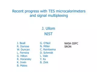
Recent progress with TES microcalorimeters and signal multiplexing J. Ullom NIST G. O’Neil N. Miller C. Reintsema D. Schmidt L. Vale Y. Xu B. Zink J. Beall R. Doriese W. Duncan L. Ferreira G. Hilton R. Horansky K. Irwin B. Mates NASA GSFC SRON
0.06 E C t= 0.04 G Temperature Resistance (W) C 0.02 C GThermal Heat Conductance 0 95.8 96 96.2 Capacity Time Temperature (mK) Transition-edge sensor (TES) calorimetry energy (x-ray) temperature response V SQUID current amp I thermometer
TES issues single pixel performance energy resolution capture efficiency speed multipixel arrays ease of fabrication, homogeneity stability of operation readout of arrays
Obstacle to better TES resolution: unexplained noise • expected noise sources: • fluctuations in thermal impedances • Johnson noise • unexpected noise source: • behaves like white voltage noise unexplained noise L/R roll-off phonon noise Johnson noise
Different TES geometries additional normal metal features definition: a = (T/R) dR/dT perpendicular bars reduce a
Noise vs. geometry: unexplained noise and a correlated all data at 60% RN • low a designs have little unexplained noise • perpendicular normal features reduce noise and a
SRON parameter study normal islands and bars … a≈ 450 a≈ 450 a≈ 500 a≈ 150 a≈40a≈40 a≈15 noise measurements to follow
Design strategy: match Eg-max to 5.9 keV, lower a a = 45 C = 0.9 pJ/K M = 1.2-1.4 1.5 mm Bi 50% at 6 keV 261 ms 400 mm
L pix2 (L pix+Lstreet)2 ~ 4 eV X-ray absorbers HgTe, … simplest absorber = material stacked on TES need mmachined collimator to shield streets what is fill fraction ? for NxN array, max wires in 1 street = N (near center) demonstrated: 2 wires & spaces in 3.5 mm for N=30, min street width ~ 55 mm with litho development, ~ 25 mm ? fill fraction = 67% [83%] for 250 mm pixels = 86% [93%] for 700 mm pixels = 90% [95%] for 1 mm pixels Bi TES SiNx Si demonstrated: 2.4 eV in 250 mm device 2.9 eV in 400 mm device predict 4.5 eV in 680 mm, 6.0 eV in 830 mm
normal metal - Au absorber X-ray absorbers - mushrooms SiNx TES Bi normal metal - heat pipe Si very high fill fraction overhang can shield streets more challenging design, fabrication NIST GSFC BiCu, ~4.5 eV at 6 keV GSFC - 4 mm electroplated Au ~2.5 eV at 6 keV Tc = 65 mK, t = 7 ms
TES for 100 keV: attach bulk absorber 1 mm Sn aborber: QE = 20% at 100 keV Mo/Cu thermometer now 27 eV at 103 keV
Arrays: fabrication straightforward NIST SRON NIST GSFC
15000 DE = 4.9 eV; Number of counts = 255534; 10000 s t n u o C 5000 0 5825 5850 5875 5900 5925 Energy (eV) TES stability stable long-term operation possible … 16 hour acquisition, no gain correction DE 10% worse than in short record 3/4 hour acquisition, no gain correction no detectable drift NIST/CSTL SRON … but cannot yet be taken for granted. Requires close attention to stray RF power, stray magnetic fields, and temperature stability. Also, some dependence on device and bias point. These dependencies not yet understood.
Time-Division SQUID Multiplexing schematic data stream . . .
32:1 multiplexer chip interface chip 8 x 8 sensor array individual sensor 6.25 mm Measure many TESs in multiplexed test setup
Multiplexed x-ray calorimeter results 8- and 16-channel results 8-channel TDM 16-channel TDM
128-pixel MUX facility complete presently: g-ray mcal four 32-channel SQUID MUX chips 16 x 16 x-ray array will be tested at the end of June
Arrays lots of data: multiplexed R(T) curves • variation in transition shape variation in response • we can already engineer the transition width; soon we will engineer the transition smoothness
Future mux performance presently, cryogenic BW ~1.5 MHz and electronics BW 3 MHz (designed in 1999) we will increase system BW to 3.5 MHz … - minor adjustments and then to 12 MHz. - cold series array, electronics redesign simulated MUX performance: NeXT ? but …
New SQUIDS! gradiometric summing coils asymmetric V-F gradiometric SQUIDs • mutual inductance optimized for x-ray measurements • asymmetric V-F greater dynamic range & linearity • gradiometric design less magnetic shielding & crosstalk • (will help system engineering) • 100 mK testing in June; production run scheduled for July
Conclusions • optimism is in order - TES calorimeters continue to improve • energy resolutions < 3 eV at 5.9 keV, 27 eV at 103 keV • very promising results in complex absorber structures • mushrooms: ~ 2.5 eV • attached bulk absorbers: 27 eV (g-ray) • array fabrication feasible • some work ahead to improve homogeneity • lengthy, stable spectra feasible • some work ahead to make routine • time-domain SQUID mux works well > 196 NeXT-like pixels [1 ms] in 1 channel in 2007 ? > 32 fast pixels [50 ms] in 1 channel also very feasible does the science case justify a g-ray array ? a TES option for NeXT could be VERY large