Sensitivity of Multiple Eigenvalues and Jordan Structure in Eigenvalue Problems
This paper explores the challenges associated with computing multiple eigenvalues and the sensitivity of their Jordan canonical forms. It presents the staircase decomposition and a two-stage algorithm to determine the multiplicity structure effectively. We investigate how perturbations affect eigenvalue computations and highlight critical previous works in the field. The paper emphasizes the importance of well-posed and well-conditioned problems, underpinning the necessity for accurate solutions in numerical linear algebra. Results demonstrate effective backward error analysis and stability of computed roots.

Sensitivity of Multiple Eigenvalues and Jordan Structure in Eigenvalue Problems
E N D
Presentation Transcript
On Computing Multiple Eigenvalues, theJordan Structure andtheirSensitivity Zhonggang Zeng Northeastern Illinois University Sixth International Workshop on Accurate Solution of Eigenvalue Problems (IWASEP VI) May 23, 2006, Penn State Univ
l l l l + + + + + + + + + + + + + + + + AU = U l l l + + + l Objectives: - Multiple eigenvalues - Staircase decomposition Jordan decomposition A = XJX-1follows, if necessary - Sensitivity 1
JCF computing … … 1966: Kublanovskaya 1970: Varah 1970: Ruhe 1976: Golub & Wilkinson 1979: Van Dooren 1980: Kagstrom & Ruhe 1983: Demmel 1987: Demmel & Kagstrom 1993: Demmel & Kagstrom 1997: Edelman, Elmroth & Kagstrom … … Main difficulty: accuracy of multiple eigenvalues 2
310 0 0 0 0 0 0 0 0 0 0 0 0 0 0 0 0 0 0 0 0310 0 0 0 0 0 0 0 0 0 0 0 0 0 0 0 0 0 0 0 0310 0 0 0 0 0 0 0 0 0 0 0 0 0 0 0 0 0 0 0 0310 0 0 0 0 0 0 0 0 0 0 0 0 0 0 0 0 0 0 0 0310 0 0 0 0 0 0 0 0 0 0 0 0 0 0 0 0 0 0 0 0310 0 0 0 0 0 0 0 0 0 0 0 0 0 0 0 0 0 0 0 0310 0 0 0 0 0 0 0 0 0 0 0 0 0 0 0 0 0 0 0 0310 0 0 0 0 0 0 0 0 0 0 0 0 0 0 0 0 0 0 0 0310 0 0 0 0 0 0 0 0 0 0 0 0 0 0 0 0 0 0 0 030 0 0 0 0 0 0 0 0 0 0 0 0 0 0 0 0 0 0 0 0 0310 0 0 0 0 0 0 0 0 0 0 0 0 0 0 0 0 0 0 0 0310 0 0 0 0 0 0 0 0 0 0 0 0 0 0 0 0 0 0 0 0310 0 0 0 0 0 0 0 0 0 0 0 0 0 0 0 0 0 0 0 0310 0 0 0 0 0 0 0 0 0 0 0 0 0 0 0 0 0 0 0 0310 0 0 0 0 0 0 0 0 0 0 0 0 0 0 0 0 0 0 0 0310 0 0 0 0 0 0 0 0 0 0 0 0 0 0 0 0 0 0 0 030 0 0 0 0 0 0 0 0 0 0 0 0 0 0 0 0 0 0 0 0 0310 0 0 0 0 0 0 0 0 0 0 0 0 0 0 0 0 0 0 0 0310 0 0 0 0 0 0 0 0 0 0 0 0 0 0 0 0 0 0 0 0310 0 0 0 0 0 0 0 0 0 0 0 0 0 0 0 0 0 0 0 031 0 0 0 0 0 0 0 0 0 0 0 0 0 0 0 0 0 0 0 0 03 JCF Ill-posed Problem: Jordan Canonical Form (JCF) 0 10 3 0 -1 -1 -4 0 0 -5 -5 0 1 0 0 -1 0 -5 -1 0 -3 -1 0 5 9 -1 3 -2 -1 1 1 -2 -2 1 -1 1 1 2 -1 -1 1 0 -1 1 3 1 7 2 -2 -11 1 0 6 -4 -3 6 0 5 -1 0 -3 -2 -1 0 0 0 -1 1 5 2 3 1 -1 0 0 0 0 0 -1 0 1 2 0 0 1 0 -1 1 -4 -2 -9 -2 6 19 -2 0 -8 8 6 -8 1 -7 1 -2 4 4 2 0 0 -1 0 -1 1 -1 1 2 1 1 0 0 0 0 0 0 1 0 0 0 0 0 0 0 0 1 9 -2 4 -3 3 3 1 -2 -2 1 0 1 2 1 -1 -1 1 0 -1 0 1 0 1 0 0 -2 0 3 4 0 0 3 0 2 0 0 -1 0 0 0 0 0 1 -4 -2 0 1 4 1 0 3 5 4 0 -2 0 0 1 0 3 1 0 1 1 -1 1 -2 1 -1 3 -1 -1 -3 3 0 -3 0 -2 -1 0 1 0 0 0 0 0 5 2 6 2 -3 -16 1 0 12 -5 -1 12 0 9 -1 0 -5 -3 -2 0 0 0 -1 4 0 1 -2 -4 -1 0 0 -5 -4 3 4 0 -1 -2 0 -3 -1 0 -1 -2 1 0 1 0 0 -2 0 0 2 0 0 2 3 2 0 0 -1 0 0 0 0 0 0 -1 4 -3 3 -1 1 1 0 0 0 0 -2 3 3 1 0 0 0 0 0 1 0 2 12 -1 2 -7 0 0 2 -4 -3 2 -3 2 4 6 -1 -2 0 0 -1 3 -4 -1 -5 -2 2 12 -1 0 -7 4 3 -7 0 -6 1 3 4 2 1 0 0 0 0 11 8 1 -2 -12 -3 0 6 -9 -8 6 1 5 0 -1 0 -7 -2 0 -3 -1 -2 0 7 -2 5 1 -1 1 -2 0 0 -2 0 -1 1 1 0 4 3 -1 -1 0 3 2 6 2 -2 -7 1 0 2 -5 -4 2 -2 2 0 3 -1 -3 1 2 0 2 5 -12 -10 2 -3 1 5 -1 0 6 6 0 0 0 -2 -1 0 6 0 3 5 0 4 -9 0 1 0 1 4 -1 0 4 4 0 -4 0 0 4 0 4 0 1 6 4 2 0 2 0 0 -3 0 0 3 0 0 3 0 3 0 0 -2 0 0 0 0 3 3
The computed roots: + + + + Ill-posed problem: root-finding with coefficients in hardware precision: 4
William Kahan (1972) They are sensitive to arbitrary perturbation, but may not be sensitive to structure preserving perturbation. Are multiple roots/eigenvalues really sensitive to perturbations? 5
perturbed polynomial p original polynomial q projected polynomial with computed roots pejorative manifold A two staged algorithm: Determine the multiplicity structure (or manifold) Reformulate / solve least squares problem well-posed, and even well conditioned 6
Stage II results: The backward error: 6.16 x 10⁻¹⁶ Refined roots 1.000000000000000 1.999999999999997 3.000000000000011 3.999999999999985 For polynomial with (inexact ) coefficients in machine precision Stage I results: The backward error: 6.05 x 10⁻¹⁰ Computed roots multiplicities 1.000000000000353 20 2.000000000030904 15 3.000000000176196 10 4.000000000109542 5 ACM TOMS, 2004: Z. Zeng, Algorithm 835 -- MultRoot Math. Comp. 2005: Z. Zeng, Computing multiple roots of inexact polynomials 7
l 1 l 1 l l 1 l J = l 1 l l l l l l + + + + + + + + + + + + + + + + Kublanovskaya (1966) Ruhe, Kagstrom, Wilkinson,Golub, Demmel, … lI+S= l l l + + + l Staircase form with Weyr characteristics: [4,3,1] JCF computing: For a given matrix A Jordan form with Segre characteristics: [3,2,2,1] find X, J: AX = XJ find U, S, l AU = U(lI+S), UHU=I 8
AY- Y(lI+S) = 0 C*Y – I = 0 is nonsingular if the Jordan structure is correct (Zeng and Li) The problem is well-posed, may even well-conditioned 9
Gauss-Newton iteration on system Example: A 50x50 matrix with eigenvalues 1, 2, 3 with multiplicity 20, 15, 5 respectively 10
A two-stage strategy for computing JCF: Stage I: determine the Jordan structure and an initial approximation Stage II: Solve the reformulated least squares problem at each eigenvalue, subject to the structural constraint, using the Gauss-Newtion iteration. 11
Minimal polynomials: A rank/nulspace problem eigenvalue Segre characteristics l1 5 3 2 2 l2 3 3 1 l3 2 ---------------------------------------------------------------------------------------------------------------------------------------------------- 10 6 3 2 Let v be a coefficient vector of p1. Then for a random x 12
leads to p2(l), p3(l), … recursively Rank/nulspace leads to p1(l) (the 1st minimal polynomial) By a Hessenberg reduction, with A1 = A, and a randomx being the first column of Q, 13
Minimal polynomials Ill-posed root-finding with approximate data Root-finding JCF structure Computing multiple roots of inexact polynomials, Z. Zeng, Math Comp 2005 Rank-revealing 14
Example: 100x100 matrix A with multiple eigenvalues 1, -1, 2, -2 50 simple eigenvalues: random 15
-- space of matrices perturbed matrix original matrix “nearest” matrix on P manifold When matrix A is possibly approximate: Stage I: Determine the manifold (matrix bundle) Stage II: Solve the well-posed least squares problem 16
has some known weaknesses • may substantially underestimate the error • may fail to discriminate a multiple eigenvalue Sensitivity of an eigenvalue(simple or multiple) Condition number At a multiple eigenvalue, k(l)= infinity by definition, not by computation 17
Error estimate = 0.0000042 Actual error = 0.0022 The condition number fails to reveal ill-posedness Example: >> eig(A) ans = 2.00078250207872 + 0.00056834208954i 2.00078250207872 - 0.00056834208954i 1.99970128002318 + 0.00092011990651i 1.99970128002318 - 0.00092011990651i 1.99903243579620 2.00000000000000 >> eig(A+E) ans = 1.99785628939037 1.99891738496176 + 0.00185657043184i 1.99891738496176 - 0.00185657043184i 2.00107196168888 + 0.00187502026186i 2.00107196168888 - 0.00187502026186i 2.00216501730835 >> norm((x*y')/(x'*y)) ans = 14.04290360613186 18
Condition number log10(error bound) log10(error) Example: 19
For l = 0: Demmel’s bound (1987) Wilkinson’s bound (1984) For l = 0.1: Kahan’s bound (1972) What is the minimum perturbation ||E|| such that an eigenvalue of A increases its multiplicity? 20
Wanted: a measurement of sensitivity • reliable in identifying a multiple eigenvalue • can be estimated/computed efficiently 21
cost: O(n2) At an eigenpair ( l , x ) ofA, define a condition number t(l) = infinity at a multiple eigenvalue the distance ||E|| to the nearest bundle with l being a double eigenvalue speculation: 22
Condition numbers Condition numbers Example: log10 (new error bound) log10(error bound) log10(error) Example: >> eig(A) ans = 2.00078250207872 + 0.00056834208954i 2.00078250207872 - 0.00056834208954i 1.99970128002318 + 0.00092011990651i 1.99970128002318 - 0.00092011990651i 1.99903243579620 2.00000000000000 23
define If A+E is the nearest matrix with (m+1)-fold l if multiplicity m is wrong Sensitivity of an m-fold eigenvalue After obtaining an m-fold eigenvalue l in staircase decomposition 24
Staircase decomposition for a double eigenvalue: -0.00000000025159 0.00000003957120 -0.00000000049184 -0.00000098980397 0.00000008765356 0.00001538421795 -0.00000205331981 -0.00017578611054 0.00003066233014 0.00154219061561 -0.00033766919246 -0.01044234247091 0.00284564181729 0.05361151873827 -0.01836110020880 -0.19998617218797 0.08857192169246 0.49723892540802 -0.30283241761169 -0.66937659896642 0.65751125003779 0.13279795424950 -0.68394528652648 0.49403745520757 -0.00000000025159 0.00000003957120 -0.00000000049184 -0.00000098980397 0.00000008765356 0.00001538421795 -0.00000205331981 -0.00017578611054 0.00003066233014 0.00154219061561 -0.00033766919246 -0.01044234247091 0.00284564181729 0.05361151873827 -0.01836110020880 -0.19998617218797 0.08857192169246 0.49723892540802 -0.30283241761169 -0.66937659896642 0.65751125003779 0.13279795424950 -0.68394528652648 0.49403745520757 0.03864934375529 -0.88858158392945 0 0.03864934375529 = F Example: 12x12 Frank matrix Eigenvalue Condition number 0.03102744447368 18281388.1 0.04950888583700 38773448.2 0.08122648015585 26647311.8 0.14364690493016 6701300.4 0.28474967198534 560311.0 0.64350532103739 14466.8 1.55398870911557 216.1 3.51185594858010 6.9 6.96153308556711 1.7 12.31107740086854 3.1 20.19898864587709 5.0 32.22889150157213 3.3 >> F = frank(12) F = 12 11 10 9 8 7 6 5 4 3 2 1 11 11 10 9 8 7 6 5 4 3 2 1 0 10 10 9 8 7 6 5 4 3 2 1 0 0 9 9 8 7 6 5 4 3 2 1 0 0 0 8 8 7 6 5 4 3 2 1 0 0 0 0 7 7 6 5 4 3 2 1 0 0 0 0 0 6 6 5 4 3 2 1 0 0 0 0 0 0 5 5 4 3 2 1 0 0 0 0 0 0 0 4 4 3 2 1 0 0 0 0 0 0 0 0 3 3 2 1 0 0 0 0 0 0 0 0 0 2 2 1 0 0 0 0 0 0 0 0 0 0 1 1 + R 25
Frank matrix is near matrices of an eigenvalue with multiplicity m = 2, l = 0.03864934375529, distance = 3.9e-12, t2(l) = 1.34e+07 m = 3, l = 0.05043386836727, distance = 4.7e-10, t3(l) = 2.73e+05 m = 4, l = 0.07030194271661, distance = 3.9e-08, t4(l) = 9.04e+03 m = 5, l = 0.10767505748315, distance = 2.1e-06, t5(l) = 5.40e+02 m = 6, l = 0.18704749378810, distance = 7.1e-05, t5(l) = 6.48e+01 26
Condition estimator - Approximate (or power iteration) - QR decomposition Q R = - Inverse iterations: - Condition number: 27