Karmarkar Algorithm
Karmarkar Algorithm. Anup Das, Aissan Dalvandi, Narmada Sambaturu, Seung Min, and Le Tuan Anh. Contents. Overview Projective transformation Orthogonal projection Complexity analysis Transformation to Karmarkar’s canonical form. LP Solutions. Simplex Dantzig 1947 Ellipsoid


Karmarkar Algorithm
E N D
Presentation Transcript
Karmarkar Algorithm Anup Das, Aissan Dalvandi, Narmada Sambaturu, SeungMin, and Le Tuan Anh
Contents • Overview • Projective transformation • Orthogonal projection • Complexity analysis • Transformation to Karmarkar’s canonical form
LP Solutions • Simplex • Dantzig 1947 • Ellipsoid • Kachian 1979 • Interior Point • Affine Method 1967 • Log Barrier Method 1977 • Projective Method 1984 • NarendraKarmarkar form AT&T Bell Labs
Linear Programming General LP Karmarkar’s Canonical Form M Subject to M Subject to • Minimum value of is 0
Karmarkar’s Algorithm • Step 1: Take an initial point • Step 2: While • 2.1 Transformation: such that is center of • This gives us the LP problem in transformed space • 2.2 Orthogonal projection and movement: Project to feasible region and move in the steepest descent direction. • This gives us the point • 2.3 Inverse transform: • This gives us • 2.4 Use as the start point of the next iteration • Set
Step 2.1 • Transformation: such that is center of - Why?
Step 2.2 • Projection and movement: Project to feasible region and move in the steepest descent direction - Why? Projection of to feasible region
Karmarkar’s Algorithm • Step 1: Take an initial point • Step 2: While • 2.1 Transformation: such that is center of • This gives us the LP problem in transformed space • 2.2 Orthogonal projection and movement: Project to feasible region and move in the steepest descent direction. • This gives us the point • 2.3 Inverse transform: • This gives us • 2.4 Use as the start point of the next iteration • Set
Projective Transformation • Transformation: such that is center of Transform
Projective transformation • We define the transform such that • We transform every other point with respect to point Mathematically: • Defining D = diag • projective transformation: • inverse transformation
Problem transformation: • projective transformation: • inverse transformation The new objective function is not a linear function. Minimize s.t. Minimize S.t. Transform
Problem transformation: Minimize S.t. Minimize S.t. Convert
Karmarkar’s Algorithm • Step 1: Take an initial point • Step 2: While • 2.1 Transformation: such that is center of • This gives us the LP problem in transformed space • 2.2 Orthogonal projection and movement: Project to feasible region and move in the steepest descent direction. • This gives us the point • 2.3 Inverse transform: • This gives us • 2.4 Use as the start point of the next iteration • Set
Orthogonal Projection • Projecting onto • projection on • normalization Minimize S.t.
Orthogonal Projection • Given a plane and a point outside the plane, which direction should we move from the point to guarantee the fastest descent towards the plane? • Answer: perpendicular direction • Consider a plane and a vector
Orthogonal Projection • Let and be the basis of the plane () • The plane is spanned by the column space of ] • , so • is perpendicular to and
Orthogonal Projection • = projection matrix with respect to ’ • We need to consider the vector • Remember • is the projection matrix with respect to
Orthogonal Projection • What is the direction of? • Steepest descent = • We got the direction of the movement or projected ’ onto • Projection on
Calculate step size • r = radius of the incircle Minimize S.t.
Movement and inverse transformation Transform Inverse Transform
Contents • Overview • Projective transformation • Orthogonal projection • Complexity analysis • Transformation to Karmarkar’s canonical form
Running Time • Total complexity of iterative algorithm = (# of iterations) x (operations in each iteration) • We will prove that the # of iterations = O(nL) • Operations in each iteration = O(n2.5) • Therefore running time of Karmarkar’s algorithm = O(n3.5L)
# of iterations • Let us calculate the change in objective function value at the end of each iteration • Objective function changes upon transformation • Therefore use Karmarkar’s potential function • The potential function is invariant on transformations (upto some additive constants)
# of iterations • Improvement in potential function is • Rearranging,
# of iterations • Since potential function is invariant on transformations, we can use whereandare points in the transformed space. • At each step in the transformed space,
# of iterations • Simplifying, we get Where • For small • So suppose both and are small -
# of iterations • It can be shown that • The worst case for would be if • In this case
# of iterations • Thus we have proved that • Thus where k is the number of iterations to converge • Plugging in the definition of potential function,
# of iterations • Rearranging, we get
# of iterations • Therefore there exists some constant such that after iterations, where , being the number of bits is sufficiently small to cause the algorithm to converge. • Thus the number of iterations is in
Rank-one modification • The computational effort is dominated by: • Substituting A’ in, we have • The only quantity changes from step to step is D • Intuition: • Let and be diagonal matrices • If and are close the calculation given should be cheap!
Method • Define a diagonal matrix , a “working approximation” to in step k such that • for • We update D’ by the following strategy • (We will explain this scaling factor in later slides) • For to doif Then let and update
Rank-one modification (cont) • We have • Given , computation of can be done in or steps. • If and differ only in entry then • => rank one modification. • If and differ in entries then complexity is .
Performance Analysis • In each step: • Substituting , and , • Let call • Then Let • Then
Performance analysis - 2 • First we scale by a factor • Then for any entry I such that • We reset • Define discrepancy between and as • Then just after an updating operation for index
Performance Analysis - 3 • Just before an updating operation for index i Between two successive updates, say at steps k1 and k2 Let call Then Assume that no updating operation was performed for index I -
Performance Analysis - 4 • Let be the number of updating operations corresponding to index in steps and be the total number of updating operations in steps. • We have Because of then
Performance Analysis - 5 • Hence • So • Finally
Contents • Overview • Transformation to Karmarkar’s canonical form • Projective transformation • Orthogonal projection • Complexity analysis
Transform to canonical form General LP Karmarkar’s Canonical Form M Subject to • x M Subject to • x
Step 1:Convert LP to a feasibility problem • Combine primal and dual problems • LP becomes a feasibility problem Dual Primal M Subject to M Subject to • x Combined
Step 2: Convert inequality to equality • Introduce slack and surplus variable
Step 3: Convert feasibility problem to LP • Introduce an artificial variable to create an interior starting point. • Let be strictly interior points in the positive orthant. • Minimize • Subject to • +
Step 3: Convert feasibility problem to LP • Change of notation • Minimize • Subject to • + M Subject to • x
Step4: Introduce constraint • Let ,…,] be a feasible point in the original LP • Define a transformation • for • Define the inverse transformation • for
Step4: Introduce constraint • Let denote the column of • If • Then • We define the columns of a matrix ’ by these equations • for • = • Then
Step 5: Get the minimum value of Canonical form • Substituting • We get • Define by • Then implies