Download
1 / 13
130 likes | 290 Vues
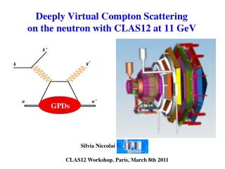
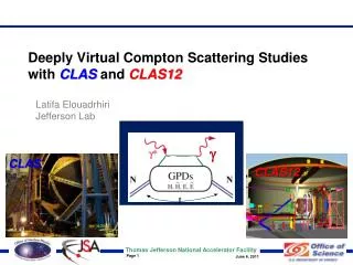
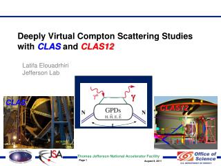
e’. ~. e. t. g. H, H, E, E (x,ξ,t). g L *. (Q 2 ). x+ξ. x-ξ. INFN Frascati, INFN Genova, IPN Orsay, LPSC Grenoble SPhN Saclay University of Glasgow. ~. p’. p. Deeply Virtual Compton Scattering on the neutron at JLab with CLAS12. CLAS12 Central Detector Meeting

E N D
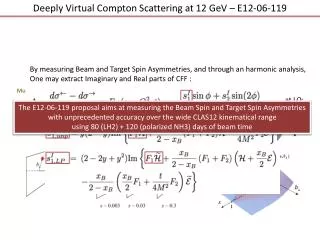
e’ ~ e t g H, H, E, E (x,ξ,t) gL* (Q2) x+ξ x-ξ INFN Frascati, INFN Genova, IPN Orsay, LPSC Grenoble SPhN Saclay University of Glasgow ~ p’ p Deeply Virtual Compton Scatteringon the neutron at JLab with CLAS12 CLAS12 Central Detector Meeting Saclay, 12/02/09 CLAS12 Workshop, Genova, 2/27/08 S. Niccolai, IPN Orsay
nDVCS with CLAS12: kinematics Physics and CLAS12 acceptance cuts applied: W> 2 GeV2, Q2 >1 GeV2,–t < 1.2 GeV2 5° < qe < 40°, 5° < qg < 40° DVCS/Bethe-Heitler event generator with Fermi motion, Ee = 11 GeV (Grenoble) <pn>~ 0.4 GeV/c More than 80% of the neutrons have q>40° → Neutron detector in the CD is needed! CD Detected in forward CLAS Not detected ed→e’ng(p) Detected in FEC, IC PID (n or g?), p, angles to identify the final state pμe + pμn + pμp = pμe′ + pμn′ + pμp′ + pμg In the hypothesis of absence of FSI: pμp = pμp’ → kinematics are complete detecting e’, n (p,q,f), g FSI effects can be estimated measuring eng, epg, edg on deuteron in CLAS12 (same experiment)
CND: constraints & design Central Tracker CTOF CND • limited space available (~10 cm thickness) • limited neutron detection efficiency • no space for light guides • compact readout needed • strong magnetic field (~5 T) • magnetic field insensitive photodetectors (APDs, SiPMs or Micro-channel plate PMTs) • CTOF can also be used for neutron detection • Central Tracker can work as a vetofor charged particles MC simulations done for: • efficiency • PID • angular resolutions • reconstruction algorithms • background studies Detector design under study: scintillator barrel
Simulation of the CND y x z • Geometry: • Simulation done with Gemc (GEANT4) • Includes the full CD • 4 radial layers (or 3, if MCP-PMTs are used) • 30 azimuthal layers (can still be optimized) • each bar is a trapezoid (matches CTOF) • inner r = 28.5 cm, outer R = 38.1 cm Reconstruction: • Good hit: first with Edep > threshold • TOF = (t1+t2)/2, with t2(1) = tofGEANT+ tsmear+ (l/2 ± z)/veff • tsmear = Gaussian with s= s0/√Edep (MeV) • s0 = 200 ps·MeV ½→ σ ~ 130 ps for MIPs • β = L/T·c, L = √h2+z2 , h = distance between vertex and hit position, assuming it at mid-layer • θ = acos (z/L), z = ½ veff (t1-t2) • Birks effect not included (will be added in Gemc) • Cut on TOF>5ns to remove events produced in the magnet and rescattering back in the CND
CND: efficiency, PID, resolution Layer 2 Layer 1 Layer 3 Layer 4 Efficiency ~ 10-16% for a threshold of 5 MeV and pn = 0.2 - 1 GeV/c Efficiency: Nrec/Ngen Nrec= # events with Edep>Ethr. pn= 0.1 - 1.0 GeV/c q = 50°-90°, f = 0° “Spectator” cut Dp/p ~ 5% Dq ~ 1.5° • b distributions (for each layer) for: • neutrons with pn = 0.4 GeV/c • neutrons with pn = 0.6 GeV/c • neutrons with pn = 1 GeV/c • photons with E = 1 GeV/c • (assuming equal yields for n and g) n/g misidentification for pn≥ 1 GeV/c
CLAS 12 Recent measurements at OrsayCEA – Orme des MerisiersDec. 2-3, 2009 B. Genolini, T. Nguyen Trung, J. Pouthas http://ipnweb.in2p3.fr/~detect
Main issues • Requested time resolution < 200 ps RMS • Plastic scintillator (best ≈2.5 ns FWHM) • Large number of photoelectrons: > 100 • High magnetic field (5T): no PMT • SiPM (MPPC, GAPD, etc.) • APD • MCP PMT • 60-cm long scintillator: • Important light losses (wrapping, absorption) • Spread of the photon time distribution Plastic scintillator (BC408) w h l = 60 cm
The test bench at Orsay Reference readout PMT (XP20D0) Coincidence scintillators • Scintillator: 60×3×3 cm^3, BC408 • Trigger: the time reference is taken from the thickest scintillator, validated by the coincidence of the two others • Mobile support to scan the scintillator • Test readout: PMT as the reference, or SiPM (in a box, for shielding) Mobile support Trigger scintillator Test readout: PMT or SiPM Test Ref Trig
Results Thi Nguyen Trung Bernard Genolini S. Pisano J. Pouthas Single pe Test σ2test =1/2 (σ2test,trig + σ2test,ref − σ2ref,trig) Ref Trig • Test = 1 SiPM Hamamatsu • (MPPC 1x1 mm2) • sTOF ~ 1.8 ns • rise time ~ 1 ns • nphe ~1 • Test = PMT • sTOF < 90 ps • nphe ~1600 • Test = 1 SiPM Hamamatsu • (MPPC 3x3mm2) • rise time ~5 ns (> capacitance) • more noise than 1x1 mm2 • Test = 1 APD Hamamatsu • (10x10 mm2 ) • sTOF ~ 1.4 ns • high noise, high rise time • Test = 1 MCP-PMT Photonis/DEP • (two MCPs) • sTOF ~ 130 ps • tested in B field at Saclay • (end of November)
Extruded scint. + WLS fiber Typical signals • Extruded scintillator made at Triumph • Wavelength shifting fiber (best results with multi cladding): > 10 pe • Measurement with a 1×1 m2 MPPC (Hamamatsu SiPM) and a PMT (Photonis XP20D0) • Time resolution: 1.4 ns RMS 100 ns PMT averaged signal 20 ns
MCP-PMT • Double-stage MCP (Photonis-DEP) • Time resolution without magnetic field = 130 ps • Test at CEA under magnetic field: not working at 5 T (amplitude ratio = 10-4)
Simulation of the light collection Simulations with Litrani Pulse shapes Relative light yields Scint. 2 2 layers Scint. 1 Prototype (0 layer) Scint. 1 Scint. 2 3 layers Adjusted on the Prototype measurements Scint. 3 Time resolution along the scintillator length
Issues 1/Can we obtain ~150 ps time resolution give the existing constraints ? (B-field, space, photodetector lifetime,…) ? (3m MCP-PMTs, APDs, SiPMs,…) 2/If not, can we afford to give up on the TOF measurement ? TOF measurement has three purposes: A/n/g separation B/ pn measurement C/ q measurement Energy deposition profile (1cm2 scintillator trapezoids) ? Preshower ? Pulse shape analysis ? Could measuring only (pe,qe,fe), (pg,qg,fg),(qn,fn) be enough ? Additional segmentation in q 3/Measuring the recoil proton instead ?