Download
1 / 50
530 likes | 834 Vues
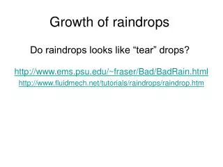
Growth of raindrops. Do raindrops looks like “tear” drops?. http://www.ems.psu.edu/~fraser/Bad/BadRain.html http://www.fluidmech.net/tutorials/raindrops/raindrop.htm. Initiation of rain in warm clouds.

E N D
Growth of raindrops Do raindrops looks like “tear” drops? http://www.ems.psu.edu/~fraser/Bad/BadRain.html http://www.fluidmech.net/tutorials/raindrops/raindrop.htm
Initiation of rain in warm clouds • Fact: The observed time scale for growth of precipitation to raindrop size (d ~ 1 mm) is about 20 min. • A significant amount of rain in the tropics originates from shallow (warm) clouds (T > 0 C). • Once raindrops attain a radius of 20 mm, growth by collision-coalescence becomes more probable (observations and theory). • For drop diameters > 30 mm, coalescence is the dominant process of drop growth (to be demonstrated).
What mechanism(s) produce drops with r > 20 mm? • Mixing between cloud and environment: • Homogeneous mixing: mixing is complete, leads to a homogeneous mixed volume of similar e/es • Inhomogeneous mixing: evaporation is local and leads to volumes of air with no or very few drops; then subsequent mixing occurs and reduces Nd; these drops can grow via larger (S-1) • Recall the sources and sinks of S from the dS/dt equation • Cloud top vs lateral mixing • Mixing (evaporation) has the largest impact on the smallest drops. Why? • The net effect is to reduce the drop concentration. How would this impact subsequent growth?
Collection • Growth process resulting from drop (or ice particle) collisions and subsequent coalescence
The continuous collection model • Important aspects: • Drop terminal fall speeds • Collision efficiency • Growth equations (models) • Continuous collection model (Bowen model) • Statistical growth (Telford model) • Statistical growth (stochastic collection model) • Condensation + stochastic collection VT A grazing trajectory for the collected drop (rs) as the flow field around the collector drop (r1) tends to move the smaller drop aside. Only those drops whose centers lie within the distance R of the fall axis of the collector drop are assumed to be collected. Fig. 7.1 from Young (1993)
Flow regimes about a sphere, as a function of Reynolds number* Fig. 7.2 from Young (1993) Laminar flow (low Re) Turbulent flow and separation (high Re) 20<Re<200 (flow separation) Re = 0 300<Re<450 (vortex loops, nonsteady) 0<Re<20 (asymmetric) Re>450 (turbulent wake) • Re = 2rVTr/m • r is given in m
Computed shapes of freely falling water drops at terminal velocity in air for diameters shown. Taken from Fig. 7.3 of Young (1993) who adapted it from Beard and Chuang (1987). Note: drops are spherical for diameters 1 mm. Oblate spheroid shape for large drops
Terminal fall speeds (pp. 124-125) • Force balance: gravity vs. frictional drag • Drag: Fdrag = (p/2)r2VT2rCDFdrag = 6pmrVT(CDRe/24) (Re = 2rVTr/m) • Gravitational force: Fg = mg = (4/3)pr3(rL-rair), or since rL >> rair, Fg = (4/3)pr3grL Drop falling at VT
Terminal fall speeds of drops • a) Stokes Law regime (r < 30 mm) • b) Intermediate drop sizes • (40 mm < r < 0.6 mm) • VT = k3r, k3 = 8x10³ s-1 (8.8) • Large drop sizes (0.6 mm < r < 2 mm) • VT = k2r1/2, k2 = 2.2x10³(r0/r)1/2 cm1/2 s-1 (8.6) (8.5)
drizzle Large raindrop Small raindrop asymptote Sea level: p = 1013.25 hPa, T = 20 C
Collision efficiency Definition: Fraction of droplets with radius r (rs) in the path (defined by airflow around the falling drop and inertial effects of the small drop) swept out by the collector drop of radius R. E(R,r) = x02 / (R + r)2 R VT Limiting trajectory associated with a glancing collistion x
E(R,r) = x02 / (R + r)2 Low for small values of r/R (small r) Drops with small r have very small inertia and follow airflow. Relative maxima near r/R = 0.6 for intermediate sizes of R > 20 mm. Also, large gradient in E near r=20 mm. This is explains why coalescence is not effective until droplet sizes attain r=20 mm. Effect at large r/R ~ 1: wake capture.
Collision efficiency as a function of R and r, based on the data in Table 8.2. Contours are values of the E. Fig. 8.3 from R&Y Small droplets (r) need to be larger the several mm in order for E to be sufficiently large. The optimum large drop (R) appears to be about 700 mm, or 0.7 mm
Coalescence efficiency (from Young 1993) Collection efficiency = Collision efficiency X Coalescence efficiency Weber number: Ratio of dynamic pressure to pressure across a curved interface http://en.wikipedia.org/wiki/Dynamic_pressure http://en.wikipedia.org/wiki/Weber_number
Results from the Bowen model Growth Equations (8.15) (8.16) Important parameters: M, U The above approximation is valid only when the updraft U is small compared to the terminal fall speed u(R)
Fig. 8.5 from R&Y. Drop trajectories for the collision efficiencies of Table 8.2 and Fig. 8.3, assuming a coalescence efficiency of 1.0. Initial drop radius is 20 mm, cloud water content is 1 g m-3, and cloud droplet radii are 10 mm. The time scale is too large by about a factor of 2.
Most of the growth occurs as the raindrops fall These calculations demonstrate the relationship among updraft, cloud height, time for rain production, and drop size that agree at least qualitatively with observations.
Statistical growth: the Telford model The statistical-discrete capture process is crucial in the early stages of rain formation. Chances captures during the early stages of the collection process are important. Reasonable drop spectra evolved over periods of a few 10’s of minutes. Based on some assumed distribution of probability of collision. n – avg drop conc. m – number of droplets in a volume V Collected droplets of uniform size of 10 mm. Collector drops have twice the volume, r = 12.6 mm
Some early work on drop growth by stochastic collection Some results Cloud droplet distribution Raindrop distribution Initial unimodel distribution evolves to a bimodel distribution (cloud & rain drops)
Collisions between all droplet pairs • Three basic modes of collection operate simultaneously to produce large drops: • Autoconversion adds water to S2 so that the other modes can operate. • Accretion is the main mechanism for transferring water from S1 to S2. • d) Large hydrometeor self capture produces large drops quickly and is responsible for the rapid increase in rg and the emerging shape of S2. Collisions only within S1 Collisions only between S1 and S2 Initial spectrum S1: r = 10 mm, M = 0.8 g m-3 Initial spectrum S2: r = 20 mm, M = 0.2 “ “ Collisions only within S2
Condensation plus stochastic coalescence. Condensation maintains the supply of water droplets for the growing raindrops, and is important. Without condensation With condensation
Maritime cloud, with Nc = 105S0.63. The collection process removes many of the cloud droplets after 500 s (N decreases), and therefore S increases. Caclulations with condensation + coalescence Relation to dS/dt eq. Increasing Ec produces a reduction in N
Same is Fig. 8.13, except for a continental cloud, with Nc = 1450S0.84. In this case the coalescence process is not effective, and the dramatic rise in S does not occur. Collision-coalescence mechanism is not as effective in this continental case
Quasi-stochastic model Figure taken from Young (1993) This again illustrates that stochastic processes are important in the early stages of raindrop growth 12.7 mm 11.5 mm 15.3 mm
Drop size distributions (Chap. 10):What controls the shape of the distribution? Idealized DSD Measured DSD (Fig. 10.1) “autoconversion” growth N (m-3 mm-1, exponential) breakup D, mm (linear)
More on the sources/sinks • Source: autoconversion represents the appearance of drops large enough to be effect collectors (previous growth by diffusion, Chap. 7) • Growth: by collection (coalescence) (Chap. 8) • Breakup: due to hydrodynamic instability of large drops, and collisions among drops
The slope of the distribution changes (or may change) as the rainfall rate changes Distribution function, Marshall-Palmer N(D) = N0e-LD (10.1) Slope factor: L(R) = 41R-0.21 (10.2) Intercept parameter: N0 = 0.08 cm-4 (10.3) • DSD relations are based on composites of observations. There is much variability: • Geographical • Temporal / spatial Fig. 10.2, R&Y
Modes of oscillations of raindropsapplies to large raindrops
Drop breakup • Aerodynamic instability due to flow around fast-falling drop (surface tension is relatively small for large drops) • Begins to be important when D = 3 mm • Drops with D > 6 mm are unstable and have short lifetimes • Collisions among drops • Coalescence efficiency is a factor: high for R<0.4 mm and r<0.2 mm
Fig. 10.3. Coalescence efficiency as a function of drop radii, r and R. The values represent the fraction of collisions that result in coalescence. 1:1 line E′ is undefined below the red line
Fig. 10.4. Theoretical DSD produced after 30 min in a model of droplet growth that includes the effects of: Condenstation Coalescence Collision breakup
Four observed modes of drop breakup: (a) filament, (b) sheet, (c) disk, and (d) bag. Taken from Young (1993).
The field of drop breakup probabilities based theory (consideration of collision kinetic energy). Dots represent where observed values exist. Taken from Young (1993).
Measurements of raindrops • Aircraft probes • Ground-based instrumentation • Disdrometers • Momentum impact • optical • Radar • Doppler • Dual polarization
Laser probes measure very large raindrop in Hawaii clouds 2-3 km deep. Courtesy K. Beard.
Disdrometer Measures the momentum impact (energy) of raindrops. The impact energy is proportional to raindrop radius, assuming that the raindrops are falling at terminal speed.
OTT Parsivel disdrometer • Description • laser-based optical system for the measurement of precipitation characteristics (see 3rd bullet) • precipitation particles are differentiated and classified as drizzle, rain, sleet, hail, snow or mixed precipitation • Measurements: size and the vertical velocity of each individual precipitation particle, from which the size spectrum, precipitation rate, the equivalent radar reflectivity factor, the visibility and the kinetic precipitation energy as well as the type of precipitation (2nd bullet) are derived. http://www.ott-hydrometry.de/web/ott_de.nsf/id/pa_parsivel_e.html#
More details http://vortex.nsstc.uah.edu/mips/data/current/surface/index.html
Disdrometer measurements Fig. 7. Observed and fitted composite spectra for the profiler’s (a) shallow convective, (b) deep convective, (c) mixed stratiform–convective, and (d) stratiform rain from 6, 21, 115, and 106 spectra, respectively, for rainfall rates of 5 mm h−1. (Tokay et al. 1997)
Time dependent drop size distribution (bow echo) Approximate mode size • Drop size was largest during the initial convection accompanying the bow passage • 2. Other maximum values were obtained during convective cell passage (915 Reflectivity) • 3. As the precipitation ended drop size decreased
Radar measurements of initial raindrop formation from nucleation on giant CCN (NaCl) in FL. Define Z Fig. 13. NCAR CP2 X-band radar reflectivity evolution of two small cumulus clouds on 5 and 10 Aug 1995. Reflectivity calculated from SCMS composite droplet distributions are shown for their corresponding 0.5-km layers on (B), (C), (F), and (G). Radar scan times (UTC) and azimuth angle are shown for each panel. From Laird et al 2000.
Evolution of radar echo in shallow Hawaiin cumulus clouds. Vertical sections of radar reflectivity factor showing the evolution from just after “first echo.” These cloud systems develop large drops and Z values.
Tumbling ice Largest drops (high ZDR values) Fig. 6. (f) Vertical section along the Y"=0 cut plane. Outer solid line is the 10-dBZ contour of reflectivity. Gray scales depict ZDR starting at 0 dB and incrementing 1 dB. Arrows are cell-relative wind vectors in the Y"=0 cut plane. (g) Contours of ZDR start at 0 dB andincrement by 1 dB (note a vertical column of numbers on upper right side of figure next to the gray scale bar). Gray scale depicts LDR starting at −24 dB (outer dashed line) and increments by 3 dB. (h) As in (g) except gray scales depict A3 starting at 0.5 dB km−1 (outer dashed line) and increments by 0.5 dB km−1. Large drops and water-coated ice
Fig. 4a. Aircraft measurements of thermodynamic and microphysical parameters during cloud passes 1–3 on 23 July 1985. The top panel for each pass illustrates the size of each drop measured by the 2D-P probe during the pass as a function of time (distance along the flight path). The bottom panel shows the updraft velocity and JW measurement of cloud liquid water. FSSP cloud droplet spectra are shown to the right of the panels, and 2D-P raindrop spectra are shown on the bottom of the figure. These spectra were averaged over regions indicated by arrows on the top pass of each of the panels. Calculated reflectivities and rainfall rates are shown for each of the raindrop spectra.From Szumowskiet al 1998 Cloud drops Rain drops
Fig. 5. Raindrop axis ratios as a function of diameter. Shown are mean axis ratios (symbols) and standard deviations (vertical lines) for the aircraft observations of Chandrasekar et al. (diamonds), the laboratory measurements of Beard et al. (triangles), Kubesh and Beard (squares), and present experiment (circles). Curves are shown for the numerical equilibrium axis ratio (αN) from Beard and Chuang (1987) , the radar–disdrometer-derived axis ratios of Goddard and Cherry (1984) , the empirical formula (αW) from the wind tunnel data of Pruppacher and Beard (1970) , and the present fit to axis ratio measurements (αA). The shaded region covers the range for previous estimates of the equilibrium axis ratio (see Table 3 ). From Andsager et al 1999.
Radar ARMOR - Advanced Radar for Meteorological and Operational Research C-band (5.5 GHz frequency, 5.5 cm wavelength) dual polarization MAX - Mobile Alabama X-band X-band (9.4 GHz frequency, 3.3 cm wavelength) dual polarization Radar equation Radar reflectivity factor Use of radar to infer rainfall rate horizontal polarization only dual polarization Vertically-pointing radar measurements
Homework Chapter 8: 8.1, 8.2, 8.4 Chapter 10: 10.3 (optional extra credit for 441 students)