Download
1 / 58
610 likes | 768 Vues
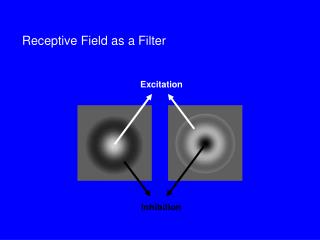
Excitation. Inhibition. Receptive Field as a Filter. pré-motrice. endogène. verbale. R. S. BOITE NOIRE. Lois / Contraintes physiques Invariants. motrice. exogène. verbale. Niveaux de traitement : Bas / Moyen / Elevé Mécanismes / Filtres / Processus / Algorithmes / Réseaux

E N D
Excitation Inhibition Receptive Field as a Filter
pré-motrice endogène verbale R S BOITE NOIRE Lois / Contraintes physiques Invariants motrice exogène verbale Niveaux de traitement : Bas / Moyen / Elevé Mécanismes / Filtres / Processus / Algorithmes / Réseaux Décisions / Biais / Expérience / Inférences / Référentiels / Contexte
Dans un système linéaire, mesurer l’amplitude du signal de sortie du système pour une amplitude d’entrée constante (l’approche de l’ingénieur) est équivalent à mesurer l’amplitude entrante requise afin d’obtenir un signal de sortie constant (l’approche du psychophysicien).
FILTRAGE MULTIECHELLE Face & SF Face, SF & Ori
1 1 1 1 1 1 1 1 2 34 2 34 5 5 5 5 5 5 5 5 -1 -1 3 3 -1 -1 Champ récepteur Réponse impulsionnelle 3 -1 -1 3 -1 1 1 1 1 0 0 2 2 3 3 4 4 6 6 5 5 5 5 -1 3 -1 3 -1 -1 -2 6 -2 -3 9 -3 -5 -5 15 15 -4 12 -4 -5 15 -5 -5 15 -5 CONVOLUTION -5 E(X) = Entrée (fct. de X) S(X) = Sortie (fct. de X) CR = h(x) = Réponse Implle (fct. de x)
PHYSICAL SPACE RECEPTIVE FIELD Incoming light Photoreceptors Axons RETINOTOPICAL SPACE RETINOTOPICAL SPACE Neurons Recording site La représentation d’un ensemble de points (image) PHYSICAL SPACE par un seul neurone Incoming light Photoreceptors est strictement identique à la représentation d’unpoint dans l’espacephysique Axons Neurons par l’ensemble des neurones qui le traitent. Recording site IMPULSE RESPONSE The RF is equivalent to the system’s Impulse Response Dans un système linéairerétinotopique,
REPRESENTATION ‘MULTIECHELLE’ DE CHAQUE POINT RETINIEN FOVEA Excentricité
Excitation Inhibition Receptive Field & Opponency Le traitement du Contraste par les Champs Récepteurs est une forme de « opponency ». Excitation Inhibition
Absorption normalisée des 4 « canaux » / filtres rétiniens (3 types de cônes & les batonnets)
RF in Motion Adelson, E. H. & Bergen, J. R. (1985). Spatiotemporal energy models for the perception of motion. J. Opt. Soc. Am. A 2, 284-299.
RF in Stereopsis Figure 1.The binocular fusion problem: in the simple case of the diagram shown on the left, there is no ambiguity and stereo reconstruction is a simple matter. In the more usual case shown on the right, any of the four points in the left picture may, a priori, match any of the four points in the right one. Only four of these correspondences are correct, the other ones yielding the incorrect reconstructions shown as small grey discs Figure 2.Eliminating 'false matches' in the stereo correspondence problem. A random dot stereogram at the top shows left and right eyes' images for crossed or uncrossed fusion (pair on the left or right respectively). Marr and Poggio's [10] proposal for establishing correct correspondences between dots in the two eyes' images is illustrated below, using only the dots highlighted in red (and dots from the same region of the left eye's image). The algorithm requires matches to be made between dots of the same colour, which gives rise to possible correspondences at all the nodes in the network marked by an open circle. Neighbouring matches with the same disparity support one another in the network, illustrated schematically by the green arrows (in their paper, the support extended farther). At the same time, matches along any line of sight (dotted lines) inhibit each other (since a ray reaching the eye must have come from only one surface). These constraints are sufficient to eliminate all but the correct matches, shown here along the main diagonal.
RF in Texture Double-opponency Figure 1. Generalized double opponency. (a) Classical, ON-center, OFF-surround receptive field (RF) that is both nonoriented and achromatic. If one assumes independent ON and OFF systems, such a unit can be looked on as double opponent in the polarity domain. This interpretation is made explicit on the left-hand side, where the response profile of this RF is shown. (b) Typical chromatic, double-opponent RF. A unit of this type responds positively to a red (R) light in its center and to a green (G) light in its surround and reverses polarity when the positions of the two lights are reversed. (c) Hypothetical double-opponent RF in the orientation domain that responds to either luminance or chromatic contrasts. In its center such a unit will respond positively to a vertical bar of a given polarity (eg., bright or R) and negatively to a 245° bar of the same polarity. Responses are reversed in its surround. Note that the linear superposition of the two groups of three RF's (in the center and the surround) results in many ON and OFF lobes of different strengths that are reminiscent of the RF of a complex cell. Gorea A. & Papathomas, T.V. (1993). Double opponency as a generalized concept in texture segregation illustrated with stimuli defined by color, luminance, and orientation. J. Opt. Soc. Am. A, 10, 1450-1462.
Spatial and spectral relationships among subunit groups in V1 of awake monkeys. Chen, Han, Poo & Dan (2007). Excitatory and suppressive receptive field subunits in awake monkey primary visual cortex (V1). PNAS, 104, 19120–19125. There were found up to nine subunits for each cell, including one or two dominant excitatory subunits as described by the standard model, along with additional excitatory and suppressive subunits with weaker contributions. Compared with the dominant subunits, the nondominant excitatory subunits prefer similar orientationsand spatial frequencies but have larger spatial envelopes. They contribute to response invariance to small changes in stimulus orientation, position, and spatial frequency. In contrast, the suppressive subunits are tuned to orientations 45°–90° different from the excitatory subunits, which may underlie crossorientation suppression. Together, the excitatory and suppressive subunits form a compact description of RFs in awake monkey V1, allowing prediction of the responses to arbitrary visual stimuli.
Spatial and spectral relationships among subunit groups in V1 of awake monkeys. Chen, Han, Poo & Dan (2007). Excitatory and suppressive receptive field subunits in awake monkey primary visual cortex (V1). PNAS, 104, 19120–19125. Dominant and nondominant excitatory (Ed and End) and suppressive (S) subunits of a cell. (Scale: 0.5°). Pooled spatial envelope of each group of subunits. Red, E; green, S. In E&S (all groups superimposed), yellow indicates overlap between E and S. Spatial-frequency spectrum of each subunit in A. Pooled frequency spectrum of each group. (C) Pooled spatial envelopes (upper rows) and frequency spectra (lower rows) of the three subunit groups for five cells.
RF in Stereopsis Figure 3. Horizontal cross-section of a disparity space. The constraint of uniqueness is implemented by letting all cells, along the two lines of sight, inhibit each other. Figure 4. Vertical cross-section of a disparity-space. The constraint of continuity is implemented by letting all active cells excite the cells, in neighboring columns, that representing similar binocular disparity.
RF in swarming See Couzin I. D. & Franks N. R. (2003). Self-organized lane formation and optimized traffic flow in army ants. Proceedings of the Royal Society of London, Series B, 270, 139-146
R V Un autre Le principe de l’UNIVARIANCE Réponse d’unfiltre (s/s ou autre) Intensité Intensitéou« qualité» du Stimulus « Qualité » (l) Un « canal » ou « filtre » ou « champ récepteur » I = stimulus intensity R = response Rmax = max resp. N = max slope S = semi-saturation cst. Rs = spontaneous R
Divisive inhibition Normalization works (here) by dividing each output by the sum of all outputs. RESPONSE NORMALIZATION Heeger, D.J. (1992). Normalization of cell responses in cat striate cortex. Visual Neuroscience, 9, 181-197.
LA NECESSITE D’UNE NONLINEARITE RESPONSE OFF units ON units CONTRASTE
LA NECESSITE D’UNE NONLINEARITE RESPONSE OFF units ON units CONTRASTE A B Lequel des deux carrés est le plus contrasté ?
LA NECESSITE D’UNE NONLINEARITE Selon la réponse des unités ON, ce serait B parce qu’une réponse positive et nécessairement plus grande qu’une réponse négative. RESPONSE ON units CONTRASTE A B Lequel des deux carrés est le plus contrasté ?
LA NECESSITE D’UNE NONLINEARITE Pour les mêmes raisons, les cellules OFF donneraient la « bonne » réponse, mais…. RESPONSE OFF units CONTRASTE A B Lequel des deux carrés est le plus contrasté ?
LA NECESSITE D’UNE NONLINEARITE ...se « tromperaient » pour la comparaison C-D. RESPONSE OFF units CONTRASTE C D Lequel des deux carrés est le plus contrasté ?
LA NECESSITE D’UNE NONLINEARITE (Half-way rectification) RESPONSE OFF units ON units Half-way rectification Half-way rectification CONTRASTE
RESPONSE OFF units ON units CONTRASTE Full-way rectification c.-à-d. Réponse absolue LA NECESSITE D’UNE NONLINEARITE (Full-way rectification)
STIMULUS p(‘yes’│N) = p(RN>c) Bruit Signal Oui FA Hit RÉPONSE Non CR Omiss. p(‘yes’│S) = p(RS>c) LE MODEL STANDARD :THEORIE de la DETECTION du SIGNAL p(N) p(S) CR Miss s1 PROBABABILITÉ Hits c0 FA CONTINUUM SENSORIEL R
Barlow’s (1972) single neuron doctrine Barlow, H.B. (1972). Single units and sensation: A neuron doctrine for perceptual psychology?Perception, 1, 371-394.
The relationship between the firing of single neurons in sensory pathways and subjectively experienced sensations. Five dogmas: • To understand nervous function one needs to look at interactions at a cellular level, rather than either a more macroscopic or microscopic level, because behaviour depends upon the organized pattern of these intercellular interactions. • The sensory system is organized to achieve as complete a representation of the sensory stimulus as possible with the minimum number of active neurons [sparse coding]. • Trigger features of sensory neurons are matched to redundant patterns of stimulation by experience as well as by developmental processes. • Perception corresponds to the activity of a small selection from the very numerous high-level neurons, each of which corresponds to a pattern of external events of the order of complexity of the events symbolized by a word [grand-mother cells]. • High impulse frequency in such neurons corresponds to high certainty that the trigger feature is present.
Field, D.J. & Olshausen, B.A. (2004) Sparse coding of sensory inputs. Current Opinion in Neurobiology, 14, 481–487. • Several theoretical, computational, and experimental studies suggest that • Neurons encode sensory information using a small number of active neurons at any given point in time. • This strategy, referred to as ‘sparse coding’, could possibly confer several advantages. • it allows for increased storage capacity in associative memories; • it makes the structure in natural signals explicit; • it represents complex data in a way that is easier to read out at subsequent levels of processing; • it saves energy. • Recent physiological recordings from sensory neurons have indicated that sparse coding could be an ubiquitous strategy employed in several different modalities across different organisms.
Absorption normalisée des 4 « canaux » / filtres rétiniens (3 types de cônes & les batonnets) Trois types de cônes codent pour une infinité de couleurs
Learned receptive fields Sparse representation in the output of the network. 144 pixel values contained in the patch. Example image patch used in training. Set of receptive fields that are learnt by maximizing sparseness in the output of a neural network. The network was trained on approximately half a million image patches of natural scenes. The receptive fields that emerge from training are spatially localized, oriented, and bandpass similar to cortical simple cells. Example image patch and its encoding by the sparse coding network. The bar chart directly above the image patch shows the 144 pixel values contained in the patch. These input activities are transformed into a much sparser representation in the output of the network, shown in the bar chart at the top. As the receptive fields are matched to the structures that typically occur in natural scenes, an image can usually be fully represented using a small number of active units. Field, D.J. & Olshausen, B.A. (2004) Sparse coding of sensory inputs. Current Opinion in Neurobiology, 14, 481–487.
Spatio-temporal correlation: MOTION N = 43
N = 51 p = 5/40 = .125 p = 6/35 = .17 p = 6/32 = .19 p = 37/37 = 1.00 Spatio-temporal correlation: MOTION
I. Create a random dot image. II. Copy image side by side. III. Select a region of one image. The Random Dot Stereogram is ready. IV. Shift (horizontally) this region and fill in the blank space left behind with the random dots to be replaced ahead. Spatio-temporal correlation: STEREO To “reveal” the “hidden” square the brain presumably computes the cross-correlation between the 2 images.
Perception as inference (Helmholtz, 1867) Helmholtz, H. von, (1867/1962) Treatise on Physiological Optics vol. 3 (New York: Dover, 1962); English translation by J P C Southall for the Optical Society of America (1925) from the 3rd German edition of Handbuch der physiologiscien Optik (first published in 1867, Leipzig: Voss)