Dirac Notation and Spectral decomposition
Dirac Notation and Spectral decomposition. Michele Mosca. review”: Dirac notation. For any vector , we let denote , the complex conjugate of . . We denote by the inner product between two vectors and . defines a linear function that maps .


Dirac Notation and Spectral decomposition
E N D
Presentation Transcript
Dirac Notation and Spectral decomposition Michele Mosca
review”: Dirac notation For any vector , we let denote , the complex conjugate of . We denote by the inner product between two vectors and defines a linear function that maps (I.e. … it maps any state to the coefficient of its component)
More Dirac notation defines a linear operator that maps This is a scalar so I can move it to front (I.e. projects a state to its component Recall: this projection operator also corresponds to the “density matrix” for )
More Dirac notation More generally, we can also have operators like
Example of this Dirac notation For example, the one qubit NOT gate corresponds to the operator e.g. (sum of matrices applied to ket vector) This is one more notation to calculate state from state and operator The NOT gate is a 1-qubit unitary operation.
Special unitaries: Pauli Matrices in new notation The NOT operation, is often called the X or σX operation.
Recall: Special unitaries: Pauli Matrices in new representation Representation of unitary operator
What is ?? It helps to start with the spectral decomposition theorem.
Spectral decomposition • Definition: an operator (or matrix) M is “normal” if MMt=MtM • E.g. Unitary matrices U satisfy UUt=UtU=I • E.g. Density matrices (since they satisfy =t; i.e. “Hermitian”) are also normal Remember: Unitary matrix operators and density matrices are normal so can be decomposed
Spectral decomposition Theorem • Theorem: For any normal matrix M, there is a unitary matrix P so that M=PPt where is a diagonal matrix. • The diagonal entries of are the eigenvalues. • The columns of P encode the eigenvectors.
Example: Spectral decomposition of the NOT gate This is the middle matrix in above decomposition
Spectral decomposition: matrix from column vectors Column vectors
Spectral decomposition: eigenvalues on diagonal Eigenvalues on the diagonal
Spectral decomposition: matrix as row vectors Adjont matrix = row vectors
Spectral decomposition: using row and column vectors From theorem
Verifying eigenvectors and eigenvalues Multiply on right by state vector Psi-2
Why is spectral decomposition useful? Because we can calculate f(A) m-th power Note that recall So Consider e.g.
Why is spectral decomposition useful? Continue last slide M = f(i)
“Von Neumann measurement in the computational basis” • Suppose we have a universal set of quantum gates, and the ability to measure each qubit in the basis • If we measure we get with probability We knew it from beginning but now we can generalize
Using new notation this can be described like this: • We have the projection operators and satisfying • We consider the projection operator or “observable” • Note that 0 and 1 are the eigenvalues • When we measure this observable M, the probability of getting the eigenvalue b is and we are in that case left with the state
Polar Decomposition Left polar decomposition Right polar decomposition This is for square matrices
Gram-Schmidt Orthogonalization Hilbert Space: Orthogonality: Norm: Orthonormal basis: