Download
1 / 75
760 likes | 1.02k Vues
Color and Texture Ch 6 and 7 of Shapiro. How do we quantify them? How do we use them to segment an image?. Color (Summary). Used heavily in human vision Color is a pixel property, making some recognition problems easy Visible spectrum for humans is 400 nm (blue) to 700 nm (red)

E N D
Color and TextureCh 6 and 7 of Shapiro How do we quantify them? How do we use them to segment an image?
Color (Summary) • Used heavily in human vision • Color is a pixel property, making some recognition problems easy • Visible spectrum for humans is 400 nm (blue) to 700 nm (red) • Machines can “see” much more; ex. X-rays, infrared, radio waves
Factors that Affect Perception • Light: the spectrum of energy that • illuminates the object surface • Reflectance: ratio of reflected light to incoming light • Specularity: highly specular (shiny) vs. matte surface • Distance: distance to the light source • Angle: angle between surface normal and light • source • Sensitivity how sensitive is the sensor
Difference Between Graphics and Vision • In graphics we are given values for all these parameters, and we create a view of the surface. • In vision, we are given a view of the surface, and we have to figure out what’s going on. What’s going on?
Some physics of color:Visible part of the electromagnetic spectrum • White light is composed of all visible frequencies (400-700) • Ultraviolet and X-rays are of much smaller wavelength • Infrared and radio waves are of much longer wavelength
Coding methods for humans • RGB is an additive system (add colors to black) used for displays. • CMY is a subtractive system for printing. • HSI is a good perceptual space for art, psychology, and recognition. • YIQ used for TV is good for compression.
RGB color cube • R, G, B values normalized to (0, 1) interval • human perceives gray for triples on the diagonal • “Pure colors” on corners
Color palette and normalized RGB Intensity I = (R+G+B) / 3 Normalized red r = R/(R+G+B) Normalized green g = G/(R+G+B) Normalized blue b = B/(R+G+B) Color triangle for normalized RGB coordinates is a slice through the points [1,0,0], [0,1,0], and [0,0,1] of the RGB cube. The blue axis is perpendicular to the page. In this normalized representation, b = 1 – r –g, so we only need to look at r and g to characterize the color.
Color hexagon for HSI (HSV) Hue is encoded as an angle (0 to 2). Saturation is the distance to the vertical axis (0 to 1). Intensity is the height along the vertical axis (0 to 1). H=120 is green saturation intensity hue I=1 H=0 is red H=180 is cyan H=240 is blue I=0
Editing saturation of colors (Left) Image of food originating from a digital camera; (center) saturation value of each pixel decreased 20%; (right) saturation value of each pixel increased 40%.
YIQ and YUV for TV signals • Have better compression properties • Luminance Y encoded using more bits than chrominance values I and Q; humans more sensitive to Y than I,Q • Luminance used by black/white TVs • All 3 values used by color TVs • YUV encoding used in some digital video and JPEG and MPEG compression
Conversion from RGB to YIQ An approximate linear transformation from RGB to YIQ: We often use this for color to gray-tone conversion.
CIE, the color system we’ve been using in recent object recognition work • Commission Internationale de l'Eclairage - this commission determines standards for color and lighting. It developed the Norm Color system (X,Y,Z) and the Lab Color System (also called the CIELAB Color System).
CIELAB, Lab, L*a*b • One luminance channel (L) and two color channels (a and b). • In this model, the color differences which you perceive correspond to Euclidian distances in CIELab. • The a axis extends from green (-a) to red (+a) and the b axis from blue (-b) to yellow (+b). The brightness (L) increases from the bottom to the top of the three-dimensional model.
References • The text and figures are from http://www.sapdesignguild.org/resources/glossary_color/index1.html • CIELab Color Space http://www.fho-emden.de/~hoffmann/cielab03022003.pdf • Color Spaces Transformations http://www.couleur.org/index.php?page=transformations • 3D Visualization http://www.ite.rwth-aachen.de/Inhalt/Forschung/FarbbildRepro/Farbkoerper/Visual3D.html
Colors can be used for image segmentation into regions • Can cluster on color values and pixel locations • Can use connected components and an approximate color criteria to find regions • Can train an algorithm to look for certain colored regions – for example, skin color
Color histograms can represent an image • Histogram is fast and easy to compute. • Size can easily be normalized so that different image histograms can be compared. • Can match color histograms for database query or classification.
Retrieval from image database Top left image is query image. The others are retrieved by having similar color histogram (See Ch 8).
How to make a color histogram • Make 3 histograms and concatenate them • Create a single pseudo color between 0 and 255 by using 3 bits of R, 3 bits of G and 2 bits of B (which bits?) • Use normalized color space and 2D histograms.
Apples versus Oranges H S I Separate HSI histograms for apples (left) and oranges (right) used by IBM’s VeggieVision for recognizing produce at the grocery store checkout station (see Ch 16).
Skin color in RGB space (shown as normalized red vs normalized green) Purple region shows skin color samples from several people. Blue and yellow regions show skin in shadow or behind a beard.
Finding a face in video frame • (left) input video frame • (center) pixels classified according to RGB space • (right) largest connected component with aspect similar to a face (by Vera Bakic)
Swain and Ballard’s Histogram Matchingfor Color Object Recognition (IJCV Vol 7, No. 1, 1991) Opponent Encoding: Histograms: 8 x 16 x 16 = 2048 bins Intersection of image histogram and model histogram: Match score is the normalized intersection: • wb = R + G + B • rg = R - G • by = 2B - R - G numbins intersection(h(I),h(M)) = min{h(I)[j],h(M)[j]} j=1 numbins match(h(I),h(M)) = intersection(h(I),h(M)) / h(M)[j] j=1
(from Swain and Ballard) 3D color histogram cereal box image
Results Results were surprisingly good. At their highest resolution (128 x 90), average match percentile (with and without occlusion) was 99.9. This translates to 29 objects matching best with their true models and 3 others matching second best with their true models. At resolution 16 X 11, they still got decent results (15 6 4) in one experiment; (23 5 3) in another.
Color Clustering by K-means Algorithm Form K-means clusters from a set of n-dimensionalvectors 1. Set ic (iteration count) to 1 2. Choose randomly a set of K means m1(1), …, mK(1). 3. For each vector xi, compute D(xi,mk(ic)), k=1,…K and assign xi to the cluster Cj with nearest mean. 4. Increment ic by 1, update the means to get m1(ic),…,mK(ic). 5. Repeat steps 3 and 4 until Ck(ic) = Ck(ic+1) for all k.
K-means Clustering Example Original RGB Image Color Clusters by K-Means
Texture: Ch7 • A description of the spatial arrangement of color or • intensities in an image or a selected region of an image.
Aspects of texture • Size or granularity (sand versus pebbles versus boulders) • Directionality (stripes versus sand) • Random or regular (sawdust versus woodgrain; stucko versus bricks) • Concept of texture elements (texel) and spatial arrangement of texels
Two Approaches: • Structural Approaches: Define texture primitives, texels and the spatial relationship among them. • 2. Statistical Approaches: Use statistical properties of color distribution
1. Structural Approaches: Texels • Extract texels by thresholding convolıtion or morphological operations
1. Structural Approaches Texel Based • Find the texels by simple procedures • Get the Voronoi tessalations: Define perpendicular bisector between the texels P and Q as
Problem with Structural Approach How do you decide what is a texel? Ideas?
2. Statistical ApproachesNatural Textures from VisTex grass leaves What/Where are the texels?
2. Statistical Approaches • Segmenting out texels is difficult or impossible in real images. • Numeric quantities or statistics that describe a texture can be • computed from the gray tones (or colors) alone. • This approach is less intuitive, but is computationally efficient. • It can be used for both classification and segmentation.
Some Simple Statistical Texture Measures 1. Edge Density and Direction • Use an edge detector as the first step in texture analysis. • The number of edge pixels in a fixed-size region tells us • how busy that region is. • The directions of the edges also help characterize the texture
Two Edge-based Texture Measures 1. edgeness per unit area for a pixel p 2. edge magnitude and direction histograms Fedgeness = |{ p | gradient_magnitude(p) threshold}| / N where N is the size of the unit area Fmagdir = ( Hmagnitude, Hdirection ) where these are the normalized histograms of gradient magnitudes and gradient directions, respectively.
Original Image Frei-Chen Thresholded Edge Image Edge Image
Local Binary Pattern Measure • For each pixel p, create an 8-bit number b1 b2 b3 b4 b5 b6 b7 b8, • where bi = 0 if neighbor i has value less than or equal to p’s • value and 1 otherwise. • Represent the texture in the image (or a region) by the • histogram of these numbers. • Compute L1 distance between two histograms: 1 2 3 100 101 103 40 50 80 50 60 90 4 5 1 1 1 1 1 1 0 0 8 7 6
Fids (Flexible Image Database System) is retrieving images similar to the query image using LBP texture as the texture measure and comparing their LBP histograms
Low-level measures don’t always find semantically similar images.
Co-occurrence Matrix Features • Define a spatial relationship specified by a vector d =(dr,dc) • d(0,1) d(1,0) d(1,1) • Compute the statistics of d within an image region • Cd (i,j)indicates how many times valueico-occurs with • valuejin a particular spatial relationshipd.