Download
1 / 19
190 likes | 208 Vues
This paper presents various approaches to the problem of Galactic MHD (Magneto-hydrodynamics) using a Shell Model. It discusses the application of Shell Model in understanding MHD turbulence with rotation, cross-helicity injection, and the free decay of MHD turbulence. The paper also explores the use of a thin disk dynamo model in studying galactic phenomena.

E N D
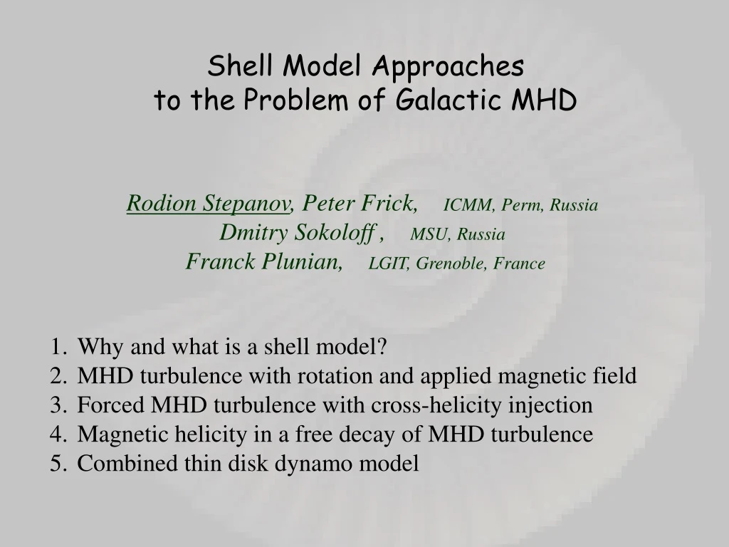
Shell Model Approaches to the Problem of Galactic MHD Rodion Stepanov, Peter Frick, ICMM, Perm, Russia Dmitry Sokoloff , MSU, Russia Franck Plunian, LGIT, Grenoble, France • Why and what is a shell model? • MHD turbulence with rotation and applied magnetic field • Forced MHD turbulence with cross-helicity injection • Magnetic helicity in a free decay of MHD turbulence • Combined thin disk dynamo model
1015 1 103 106 109 1012 1015 Rm=UL/h Interstellar medium Galaxies 10+12 1012 Convective zone The Sun 10+9 Accretion discs 109 10+6 10-3 10-6 1 Pm=10+3 106 Liquid core Jupiter 103 Liquid core The Earth DNS Experiments Liquid Na 1 Re=UL/n
Kolmogorov 41 Energy cascade Spectral flux Dissipation e e Inertial range k kn kF Large Small
Shell model of MHD turbulence Brandenburg, A. et al, 1996; Frick, P. and Sokoloff, D. 1998; Basu, A. et al 1998 Generic equations: Triadic interaction: p k q Coefficients c are derived from conservation laws (total energy, cross-helicity, magnetic helicity)
How much do we gain ? uk k -1/3 k kn kF 3D Kolmogorov Number of gridpoints per unit volume: Number of time steps: Number of timesteps x gridpoints: Shell model Number of logarithmic shells: Number of timesteps x gridpoints:
Small scale dynamo at low Pm Pm=10-3 Re=109 Eu Eb Stepanov R. and Plunian F., 2006, J. Turbulence
Phenomenology of isotropic turbulence with applied rotation and field Zhou 1995
W R RA (e /h)1/2 RKA RK e =W vA2 vA 0 (he)1/4 W= vA2 /h E(k) E(k) W 1/2 e1/2 k -2 W 1/2 e1/2 k -2 vA1/2 e1/2 k -3/2 e2/3 k -5/3 R A E (k) R K E(k) W1/2 e1/2 k -2 W1/2e1/2k-2 vA /h W /vA (e /h3)1/4 (W 3/e)1/2 e2/3 k -5/3 vA1/2 e1/2 k -3/2 R R K A (W3/e)1/2 e /vA3 vA /h (W/h)1/2
E(k) E(k) W 1/2 e1/2 k -2 W 1/2 e1/2 k -2 vA1/2 e1/2 k -3/2 e2/3 k -5/3 R A R K E(k) W1/2 e1/2 k -2 vA /h W /vA (e /h3)1/4 (W 3/e)1/2 e2/3 k -5/3 vA1/2 e1/2 k -3/2 R K A (W3/e)1/2 e /vA3 vA /h Plunian F. and Stepanov R. 2010, PRE
Energy spectra for different cross helicity input rate Energy injection rate – e=1 Cross-helicity injection rate – c<1 Normalized spectra Spectral index versus c k k c The stationary input of cross-helicity strongly affects the small-scale turbulence: the spectral energy transfer becomes less efficient and the turbulence accumulates the total energy. Mizeva I.A. et al, 2009, Doklady Physics
Long-term free decay 128 runs Re=Rm=105 Evolution up to t=105 Initial conditions Normalized cross-helicityC=Hc/E First scenario: C=±1 Second scenario Frick & Stepanov 2010
Long-term free decay Cross-helicity vs time Cross-helicity spectra for different time Inverse cascade of cross-helicity
Long-term free decay • at t=100 • at t=1000 • at t=10000 Normalized magnetic helicity Cb=Hb/Eb Second scenario: Cb=±1
Mean fields (large-scale) Turbulent fields (small-scale) Coupling: small large GRID-SHELL MODEL OF TURBULENT DISK DYNAMO large small
Numerical results large-scale poloidal/toroidal magnetic field small-scale kinetic/magnetic field Energy of vs time αu≠0αb=0 D=-1 αu≠0αb=0 D=-20 αu≠0αb=0 D=-100 αu≠0αb≠0 D=-200
Global reversals Dynamical alpha-quenching log α log <B>
Conclusion remarks • Shell models have passed many tests • Shell models can be used to check phenomenological predictions • Shell models are able to give something new about MHD turbulence