Understanding Correlation and ANOVA in Data Analysis
310 likes | 414 Vues
Learn about correlation and ANOVA models in data analysis, explore their application, correlation types, ANOVA table results, assumptions, post-hoc analysis, multi-way ANOVA, testing assumptions, higher-order interactions, and an alternative approach using linear models.

Understanding Correlation and ANOVA in Data Analysis
E N D
Presentation Transcript
Data • Data is from the University of York project on variation in British liquids. • JK Local, Alan Wrench, Paul Carter
Correlation • When we have two variables we can measure the strength of the linear association by correlation • Correlation in a strict technical statistical sense is the linear relationship between two variables.
Correlation • Many times we are not interested in the differences between two groups, but instead the relationship between two variables on the same set of subjects. • Ex: Are post-graduate salary and gpa related? • Ex: Is the F1.0 measurement related to the F1.1 measurement? • Correlation is a measurement of LINEAR dependence. Non-linear dependencies have to be modeled in a separate manner.
Correlation • There is a theoretical correlation, usually represented by ρX,Y • We can calculate the sample correlation between two variables (x,y) The Pearson Coefficient is given to the left. • This will vary between • -1.0 and 1.0 indicating the direction of the relationship.
Correlation Pearson's product-moment correlation data: york.data$F1.0 and york.data$F1.1 t = 45.9262, df = 318, p-value < 2.2e-16 alternative hypothesis: true correlation is not equal to 0 95 percent confidence interval: 0.9161942 0.9452264 sample estimates: cor 0.932194
Correlation Types • Pearson’s Tau • X,Y are continuous variables. • Kendall’s Tau • X,Y are continuous or ordinal. The measure is based on X ranked and the Y ranked. The ranks are used as the basis
One-Way ANOVA • If we want to test more than two means equality, we have to use an expanded test: One-Way ANOVA
An Example • Vowels: a, i, O, u • Are the F1 measurements the same for each corresponding vowel in the segment? • Assumptions: Normality, each group (level of vowel) has the same variance, independent measurements.
Results Analysis of Variance Table Response: york.data$F1.0 Df SS MS F Pr(>F) Vowel 3 10830838 3610279 189.96 < 2.2e-16 *** Residuals 316 6005850 19006
What about the assumptions? • Can we test for equal variance? Yes. • If the variance is not equal, is there a solution that will still allow us to use ANOVA? Yes.
Post-hoc analysis • There is a difference between the mean of at least one vowel and the others, so what? • We can test where the difference is occurring through pairwise t-tests. This type of analysis is often referred to as a post-hoc analysis.
Bonferroni Pairwise comparisons using t tests with pooled SD data: york.data$F1.0 and york.data$Vowel a i O i < 2e-16 - - O < 2e-16 <2e-16 - u < 2e-16 1 6.5e-14 P value adjustment method: bonferroni
Multi-Way ANOVA • Usually we are not interested in merely one factor, but several factors effects on our independent variable. • Same principle [Except now we have several ‘between groups variables’ ]
Multi-Way ANOVA Df Sum Sq Mean Sq F value Pr(>F) Vowel 3 173482 57827 2.0353 0.1077197 Liquid 1 216198 216198 7.6092 0.0059747 ** Sex 1 340872 340872 11.9971 0.0005687 *** Residuals 634 18013735 28413
Testing Assumptions • Bartlett’s Test: • H0: All variances for each of your cells are equal. • If your p-value is significant (<.05), then you should not be using an ANOVA, but some non-parametric test that relies on ranks. • We don’t have to worry about this with large sample data. The central limit theorem states that with enough data you will eventually get normality (of the mean).
Higher Order Interactions • It often isn’t enough to test factors by themselves, but we want to model higher-order interactions. • We are looking at Sex, Liquid and Vowel– there are Sex x Liquid, Sex x Vowel, Vowel x Liquid and Sex x Liquid x Vowel as possible interaction effects.
An Alternative Approach: Linear Model • Linear Models allow for an easily expandable approach that allows us to answer questions more explicitly without having to add more machinery with each new factor or covariate. • The underlying form in an ANOVA is essentially a linear model.
What would it look like? • In a linear model, we estimate parameters (or coefficients) of the predictors on a response. • Ex: We want to model the effect of Vowels on F1.0
What are each of the pieces? • α represents the intercept term and the mean for F1.0 when the type of vowel is controlled for. • τi represents the treatment effect of the ith vowel. • ε represents the noise and is assumed to be N(0,σ2) (i.e. normally distributed with a mean of zero and constant variance).
Inestimability • We can’t really estimate all of the data in our model. • We don’t have a control group where there isn’t a vowel effect.
Two Solutions • Stick with the model. You can only test functions of the parameters and only if they are estimable [The hard way and only if you know a fair amount of linear algebra.] • Pick a control group and allow that to be your baseline (or alpha).
The Simple Way Call: lm(formula = F1.0 ~ Vowel) Residuals: Min 1Q Median 3Q Max -322.62 -109.44 -31.20 67.48 1044.13 Coefficients: Estimate Std. Error t value Pr(>|t|) (Intercept) 426.43 13.51 31.566 <2e-16 *** Voweli -42.62 19.10 -2.231 0.0260 * VowelO -33.94 19.10 -1.776 0.0761 . Vowelu -35.16 19.10 -1.841 0.0662 . --- Signif. codes: 0 '***' 0.001 '**' 0.01 '*' 0.05 '.' 0.1 ' ' 1 Residual standard error: 170.9 on 636 degrees of freedom Multiple R-Squared: 0.009255, Adjusted R-squared: 0.004582 F-statistic: 1.98 on 3 and 636 DF, p-value: 0.1157
Model Assestment • Standard F: Are any of the levels significant? • R2: How much variation in the response is explained by the predictor(s)
What’s Next? • How to handle repeated measures? • Generalized Linear Models (Counts, proportions) • Classification and Regression Trees (Decision Trees).