Download
1 / 57
570 likes | 598 Vues
Explore parallelized mesh simplification methods, focusing on R-Simp algorithm suitability, efficiency improvement, and output quality retention. Understand surface simplification and primitive removal concepts for optimizing polygonal models.

E N D
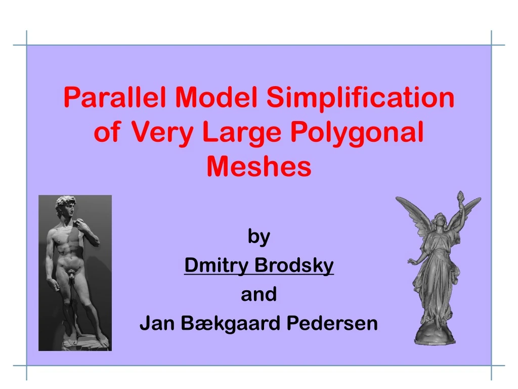
Parallel Model Simplification of Very Large Polygonal Meshes by Dmitry Brodsky and Jan Bækgaard Pedersen
What did we do? • Parallelized an existing mesh simplification algorithm • Show that R-Simp [Brodsky & Watson] is well suited for parallel environments • Able to simplify large models • Achieve good speedup • Retain good output quality 30M 20K
Computer graphics • Scenes are created from models I am the Stanford Bunny
Computer graphics • Scenes are created from models • Models are create from polygons • The more polygons the more realistic the model • Triangles are most often used • Consisting of 3 vertices specifying a face • Hardware is optimized for triangles
Why simplify? • Graphics hardware is too slow • Render ~10k polygons in real-time • Models are too large • 100k polygons or more • Highly detailed models are not always required • Trade quality for rendering speed
What is simplification? 70,000 Polygons 5,000 Polygons • Reduce the number of polygons • Maintain shape
What is simplification? 70,000 Polygons 5,000 Polygons • The desired number of polygons depends on the scene
So what’s the problem? • Models are becoming very large • Model acquisition is getting better • Simplification is time consuming • Trade-off time for quality • On the order of hours and days • Models do not fit into core memory • Algorithms require 10’s of gigabytes • 32 bits are not enough
What can we do? • Partition the simplification process into smaller tasks • Execute the tasks in parallel or sequentially • Reduce contention for core (page faults) • Not applicable to all algorithms
Surface simplification • Flat surface patches can be represented with a few polygons • Remove excess polygons by removing edges or vertices
Surface simplification • Flat surface patches can be represented with a few polygons • Remove excess polygons by removing edges or vertices
Surface simplification • Flat surface patches can be represented with a few polygons • Remove excess polygons by removing edges or vertices
Removing primitives • Remove the primitive that causes the least amount of distortion • Preserve significant features • E.g. corners
Removing primitives • Remove the primitive that causes the least amount of distortion • Preserve significant features • E.g. corners • Avoid primitives that form corners
Removing primitives • Remove the primitive that causes the least amount of distortion • Preserve significant features • E.g. corners • Avoid primitives that form corners • Choose primitives on flat patches
Conventional algorithms • Edge collapse • Iteratively remove edges [Garland & Heckbert, Hoppe, Lindstrom, Turk] • Decimation • Combine polygons, remove vertices to create large planar patches [Hanson, Schroeder] • Clustering • Spatially cluster vertices or faces • Poor quality output [Rossignac & Borrel]
Edge collapse • High quality output • Access is in distortion order
Edge collapse • High quality output • Access is in distortion order 4 2 1 3
Edge collapse • High quality output • Access is in distortion order • Edges are sorted by distortion • Can’t exploit access locality • Data can not be partitioned • O(n log n ), n is input size • Large models are problematic • Take long to simplify • Have to fit into core memory
Decimation • Good quality output • Access is in spatial order
Decimation • Good quality output • Access is in spatial order 1 2 3 4
Decimation • Good quality output • Access is in spatial order • Models are usually polygonal soups • Data reorganization is necessary to exploit access locality • Topology information is needed • Surface partitioning is unintuitive • Data has to be sorted first • Should not split planar regions
Memory efficient algorithms • Edge collapse [Lindstrom & Turk] • Cluster refinement [Garland] • Modified R-Simp • Re-organizes and clusters vertices and faces to improve memory access locality [Salamon et al.]
What do we do? • Simplify in reverse - “R”-Simp • Start with a coarse approximation and refine by adding vertices • Access in model order
What do we do? Vertices Faces x0, y0, z0 0: v1, v2, z3 x1, y1, z1 1:va, vb, vc xn, yn, zn m: vi, vj, vk • Simplify in reverse - “R”-Simp • Start with a coarse approximation and refine by adding vertices • Access in model order 1 2 3
What do we do? • Simplify in reverse - “R”-Simp • Start with a coarse approximation and refine by adding vertices • Access in model order • Can exploit access locality • Less reorganization necessary • Data intuitively partitions • Linear runtime for an output size • O(ni log no) • Produce good quality output
The algorithm • Partition the model
Initial clustering • Spatially partition into 8 clusters • Cluster: A vertex in the output model
The algorithm • Partition the model • Main loop • Choose a cluster to split
Choosing a cluster • Select the cluster with the largest surface variation (curvature).
Surface variation • Computed using face normals and face area
Surface variation • Computed using face normals and face area • curvedness = ∑normali* areai
The algorithm • Partition the model • Loop • Choose a cluster to split • Partition the cluster
Splitting a cluster • Split into 2,
Splitting a cluster • Split into 2, 4,
Splitting a cluster • Split into 2, 4, or 8 subclusters
How to split? • Split based on surface curvature • Compute the mean normal and directions of maximum and minimum curvature • Directions guide the partitioning Mean Normal Direction of Minimum Curvature Direction of Maximum Curvature
Surface types • Goal: create large planar patches • Cylindrical: partitioned into 2 • Hemispherical: partitioned into 4 • Everything else is partitioned into 8
The algorithm • Partition the model • Loop • Choose a cluster to split • Partition the cluster • Compute surface variation for subclusters • Repeat • Re-triangulate the new surface
Moving to PR-Simp • Clusters naturally partition data • Assign initial clusters to processors • Each processor refines to a specified limit • Results are reduced and the surfaces are stitched together
PR-Simp • Master - Slave configuration • The dataset is available to all processors • Current implementation uses MPI • Scales to any number of processors
Master: initialization • Determine bounding box of model • Determine initial clusters: • Axis aligned planes • # of Procs = fx x fy x fz • Slaves receive: • bounding box, fx x fy x fz, and output size • Processor ID corresponds to a unique cluster
Slave: simplification • Determine output size for cluster: Pout = Pin (Fullout / Fullin) • Read in the cluster • Store faces that span processor boundaries • Run standard R-Simp algorithm • Re-triangulate assigned portion of the simplified surface
Building the output model • Reduce the results • Slaves propagate: • The new triangulated surface • Faces that span processor boundaries • Surfaces are stitched together at each reduction step • Master outputs the simplified model
Evaluation • Ability to simplify • Some models needed more than 4GB of core • Speedup • Reduce page faulting (memory thrashing) • Little or no loss of output quality • Test bed: • 20 Pentium III 550Mhz with 512MB • Connected by 100Mbps network
Test subjects David St. Matthews Dragon 8,253,996 871,306 6,755,412 Happy Buddha Lucy Stanford Bunny Blade 1,765,388 28,045,920 69,451 1,087,474
Output quality at 20K David St. Matthews Dragon 8,253,996 871,306 6,755,412
Output quality at 20K Happy Buddha Lucy Stanford Bunny Blade 1,765,388 28,045,920 69,451 1,087,474
Sequential vs parallel quality 5K 10K 20K Sequential Parallel
Quantitative results • Simplified a 30M polygon model