Advanced 3D Photorealistic Modeling with Sensors and Coordinate Systems
240 likes | 374 Vues
This guide explores the intricate process of 3D photorealistic modeling using various sensors, including scanners and cameras. It covers the local and global coordinate systems, the calibration of cameras, and the transformation of individual scan coordinates into unified object coordinates. Detailed methodologies are discussed, such as polynomial fitting and projection transforms for high accuracy, as well as surface generation techniques using Polyworks and GoCad. The emphasis is on reducing errors through careful alignment and adjustment for precise modeling results.

Advanced 3D Photorealistic Modeling with Sensors and Coordinate Systems
E N D
Presentation Transcript
3D Photorealistic Modeling Process
Different Sensors • Scanners • Local coordinate system • Cameras • Local camera coordinate system • GPS • Global coordinate system
Coordinate Systems • Individual local scanner coordinates (each scan) • Object coordinate system (single coordinate system aligning all scans) • Camera coordinate system (each photograph) • Global coordinates
Scanner Coordinate Z • Individual scanner local coordinate • Not necessary to level Y X
Y X Z Camera Coordinate System • Each photograph has its own coordinates • Units: mm or pixel
Putting it together • From individual scan coordinates to object coordinates • From object (or global) coordinates to camera coordinates • From object coordinates to global coordinates
Individual coordinates to object coordinates (1/2) • Traditional survey approaches • Need to level the scanner • set up backsight • Knowing scanner location and backsight angle • transform each point to the object coordinate system, usually global. • Advantage: • easy to set up • one-step from local to global coordinates. • Disadvantage: • problem in generating mesh models.
From individual coordinates to object coordinates (2/2) • Use mesh alignment techniques (Polyworks) • No need to level. • Requires overlap with common features to minimize the distance. Z T = Y sc1 sc2 X
From Object to Camera (1/2) • Two approaches • Polynomial fit (rubber sheeting) • Low accuracy, • No need to know camera intrinsic parameters • Projection transform (pinhole model) • High accuracy
From Object to Camera (2/2) • From object to camera coordinate system (pin hole model) • Perspective projection to convert to image coordinates (uv, pixel, or mm) 6 unknowns assuming known f Nonlinear-needs initial value
Camera Calibration • Correct lens distortion • Radial distortion • Tangential distortion • Calculate f, k1, k2, p2, p2 in the lab for each lens.
Example of the calibration (Canon 17mm) 1 2 • Radial distortion • Tangential distortion • Complete model 3
Example Iteration = 8 Residuals pts51 = -0.0027 -0.0065 pts50 = 0.0045 0.0085 pts2034 = 0.0050 0.0087 pts 2010 = -0.0066 -0.0100 omage:0.08839938218814 phi:1.36816786714242 kappa: 1.45634479894558 X: -0.975 Y: 0.519 Z: -0.013
Bundle Adjustment Adjust the bundle of light rays to fit each photo
Bundle Adjustment (2/2) Photo no : 7735 pt no U V 14 0.003 -0.006 15 0.003 -0.001 204 -0.001 0.004 205 -0.001 0.009 16 0.017 0.005 206 0.000 0.001 207 -0.001 -0.009 208 0.001 0.010 302 -0.006 -0.009 Photo no : 7734 pt no U V 201 -0.000 -0.000 202 0.000 0.003 203 -0.000 -0.006 14 -0.003 0.012 15 0.000 0.001 204 0.001 -0.004 205 0.001 -0.009 302 0.001 0.004 Photo no omega phi kappa X Y Z 7733 3.5147 78.25411 85.03737 -1.031 0.628 0.046 7734 21.026 79.86519 68.09084 0.419 14.735 -1.055
s From Object to Global (1/2) • 7-parameter conformal transformation Where m11 = cos(phi) * cos(kappa); m12 = -cos(phi) * sin(kappa); m13 = sin(phi) m21 = cos(omega) * sin(kappa) + sin(omage) * sin(phi) * cos(kappa); m22 = cos(omage) * cos(kappa) – sin(omega) * sin(phi) * sin(kappa); m23 = -sin(omage) * cos(phi); m31 = sin(omage) * sin(kappa) – cos(omage) * sin(phi) * cos(kappa); m32 = siin(omage) * cos(kappa) + cos(omage) * sin(phi) * sin(kappa); m33 = cos(omage) * cos(phi); and s is scale factor
Transform to Global (2/2) GPS Object Iteration:5 scale : 0.998986 (*****) omega : 0.22279535 phi : -0.04740587 kappa : 1.45393837 X trans: 24.834 Y trans: 11.698 Z trans: 2.142 Pt: 1, X -0.012 Y 0.042 Z 0.010 Pt: 2, X 0.008 Y -0.004 Z -0.012 Pt: 3, X 0.011 Y 0.012 Z 0.004 Pt: 4, X -0.017 Y -0.032 Z -0.007 Pt: 5, X 0.010 Y -0.018 Z 0.006
REDUCTION TO THE ELLIPSOID D h S H N R Earth Radius 6,372,161 m 20,906,000 ft. S = D x R R + h h = N + H • R S = D x R + N + H Earth Center
REDUCTION TO GRID • Sg = S (Geodetic Distance) x k (Grid Scale Factor) • Sg = 1010.366 x 0.99991176 • = 1010.277 meters
REDUCTION TO ELLIPSOID • S = D x [R / (R + h)] • D = 1010.387 meters (Measured Horizontal Distance) • R = 6,372,162 meters (Mean Radius of the Earth) • h = H + N (H = 158 m, N = - 24 m) • = 134 meters (Ellipsoidal Height) • S = 1010.387 [6,372,162 / 6,372,162 + 134] • S = 1010.387 x 0.999978971 • S = 1010.366 meters
COMBINED FACTOR • CF = Ellipsoidal Reduction x Grid Scale Factor (k) • = 0. 0.999978971 x 0.99991176 • = 0.999890733 • CF x D = Sg • 0.999890733 x 1010.387 = 1010.277 meters
Surface Generation • Through merge process in Polyworks • Through fitting through GoCad • Through direct triangulation (Delauney triangulation, TIN)
Surface cleaning (in Polyworks) • The single most time consuming part of entire process (90% of time). • Filling the holes (because of scan shadow) • Correct triangles