Microarray Data Analysis
Microarray Data Analysis. March 2004. Differential Gene Expression Analysis. The Experiment Micro-array experiment measures gene expression in Rats (>5000 genes). The Rats split into two groups: (WT: Wild-Type Rat, KO: Knock Out Treatment Rat) Each group measured under similar conditions

Microarray Data Analysis
E N D
Presentation Transcript
Microarray Data Analysis March 2004
Differential Gene Expression Analysis • The Experiment • Micro-array experiment measures gene expression in Rats (>5000 genes). • The Rats split into two groups: (WT: Wild-Type Rat, KO: Knock Out Treatment Rat) • Each group measured under similar conditions • Question: Which genes are affected by the treatment? How significant is the effect? How big is the effect?
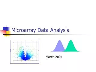
For each gene compare the value of the effect between population WT vs. KO (fold change) For each gene calculate the significance of the change (t-test, p-value) Identify Genes with high effect and high significance Volcano Plot High Significance Low Significance Fold change: 1 fold change: effect is double 2 fold change: effect is 4 times n fold change: 2 n -ve effect +ve effect Analysis Workflow The lower the p-value the higher significance (confidence) p=0.001, p=0.01, p=0.001 The more decimal places the more confident I am
Hypothesis Testing • Uses hypothesis testing methodology. • For each Gene (>5,000) • Pose Null Hypothesis (Ho) that gene is not affected • Pose Alternative Hypothesis (Ha) that gene is affected • Use statistical techniques to calculate the probability of rejecting the hypothesis (p-value) • If p-value < some critical value reject Ho and Accept Ha • The issues: • Estimation of Variance : Limited sample size (= few replicates) • Normal Distribution assumptions: Law of large number does not apply • Multiple Testing: ~10 000 genes per experiments • Need to use a t-test
Statistics 101 • Comparing Two Independent Samples • z Test for the Difference in Two Means (variance known) • t Test for Difference in Two Means (variance unknown) • F Test for Difference in two Variances • Comparing Two Related Samples: • t Tests for the Mean Difference • Wilcoxon Rank-Sum Test: • Difference in Two Medians
68% of dist. 1 s.d. 1 s.d. x The Normal Distribution Many continuous variables follow a normal distribution, and it plays a special role in the statistical tests we are interested in; • The x-axis represents the values of a particular variable • The y-axis represents the proportion of members of the population that have each value of the variable • The area under the curve represents probability – e.g. area under the curve between two values on the x-axis represents the probability of an individual having a value in that range • Mean and standard deviation tell you the basic features of a distribution • mean = average value of all members of the group • standard deviation = a measure of how much the values of individual members vary in relation to the mean • The normal distribution is symmetrical about the mean • 68% of the normal distribution lies within 1 s.d. of the mean
Any normal distribution can be transformed to a standard distribution (mean 0, s.d. = 1) using a simple transform Pdf is: Normal Distribution and Confidence Intervals a/2 = 0.025 a/2 = 0.025 1-a = 0.95 -1.96 1.96 0.025 = p-value: probability of a measurement value not belonging to this distribution
Hypothesis Testing: Two Sample Tests TEST FOR EQUAL MEANS TEST FOR EQUAL VARIANCES Ho Ho Population 1 Population 1 Population 2 Population 2 Ha Ha Population 1 Population 1 Population 2 Population 2 If standard deviation known use z test, else use t-test Use f-test
Normal Distribution vs T-distribution • t-test is based on t distribution (z-test was based on normal distribution) • Difference between normal distribution and t-distribution Normal distribution t-distribution
T-test • t-test: Single Sample vs. Multi-Sample • Multi Sample: Independent Groups vs. Paired • Are measurements in the two groups related? • What am I testing for: • Right Tail: (group1 > group2) • Left Tail: (group1 < group2) • Two Tail: Both groups are different but I don’t care how • How do I calculate p value for a t-test • Use Computer Software • Statistics Tables: • calculate t-statistic (easy formula) • then lookup p-value in table (don’t use formula to calculate !)
Single Sample t-test • t-test: Used to compare the mean of a sample to a known number (often 0). • Assumptions: Subjects are randomly drawn from a population and the distribution of the mean being tested is normal. • Test: The hypotheses for a single sample t-test are: • Ho: u = u0 • Ha: u < > u0 • p-value: probability of error in rejecting the hypothesis of no difference between the two groups. (where u0 denotes the hypothesized value to which you are comparing a population mean)
Multi-Sample: Setting Up the Hypothesis H0: m 1 - m 2£ 0 H1: m 1 - m 2> 0 H0: m 1£ m 2 H1: m 1 > m 2 Right Tail OR H0: m 1³ m 2 H0: m 1 - m 2³ 0 H1: m 1 - m 2 < 0 OR Left Tail H1: m 1 < m 2 H0: m 1 = m 2H1: m 1¹m 2 H0: m 1 -m 2 = 0 H1: m 1 - m 2 ¹ 0 Two Tail OR
Independent Group t-test • Independent Group t-test: Used to compare the means of two independent groups. • Assumptions: Subjects are randomly assigned to one of two groups. The distribution of the means being compared are normal with equal variances. • Example: Test scores between a group of patients who have been given a certain medicine and the other, in which patients have received a placebo • Test: The hypotheses for the comparison of two independent groups are: • Ho: u1 = u2 (means of the two groups are equal) • Ha: u1 <> u2 (means of the two group are not equal) • A low p-value for this test (less than 0.05 for example) means that there is evidence to reject the null hypothesis in favour of the alternative hypothesis.
Paired t-test • Paired t-test: • Most commonly used to evaluate the difference in means between two groups. • Used to compare means on the same or related subject over time or in differing circumstances. • Compares the differences in mean and variance between two data sets • Assumptions: The observed data are from the same subject or from a matched subject and are drawn from a population with a normal distribution. • Can work with very small values.
Paired t-test • Characteristics: Subjects are often tested in a before-after situation (across time, with some intervention occurring such as a diet), or subjects are paired such as with twins, or with subject as alike as possible. • Test: The paired t-test is actually a test that the differences between the two observations is 0. So, if D represents the difference between observations, the hypotheses are: • Ho: D = 0 (the difference between the two observations is 0) • Ha: D 0 (the difference is not 0)
Where d is calculated by Calculating t-test (t statistic) • First calculate t statistic value and then calculate p value • For the paired student’s t-test, t is calculated using the following formula: And n is the number of pairs being tested. • For an unpaired (independent group) student’s t-test, the following formula is used: Where σ(x) is the standard deviation of x andn (x) is the number of elements in x.
Calculating t-test (p value) • When carrying out a test, a P-value can be calculated based on the t-value and the ‘Degrees of freedom’. • There are three methods for calculating P: • One Tailed >: • One Tailed <: • Two Tailed: Where P is calculated in the following way: • The number of degrees (v) of freedom is calculated as: • UnPaired: n(x) +n (y) -2 • Paired: n- 1 where n is the number of pairs. This value should normally be greater than 1. where B is the beta function:
Calculating t and p values • You will usually use a piece of software to calculate t and P • (Excel provides that !). • You may calculate t yourself it is easy ! • You are not required to know the equations for p: • You can assume access to a function p(t,v) which calculates p for a given t value and v (number of degrees of freedom) • or alternatively have a table indexed by t and v
Reject H Reject H 0 0 .025 .025 t -2.0154 0 2.0154 t-test Interpretation • Results of the t-test: If the p-value associated with the t-test is small (usually set at p < 0.05), there is evidence to reject the null hypothesis in favour of the alternative. • In other words, there is evidence that the mean is significantly different than the hypothesized value. If the p-value associated with the t-test is not small (p > 0.05), there is not enough evidence to reject the null hypothesis, and you conclude that there is evidence that the mean is not different from the hypothesized value. Note as t increases, p decreases T (value) must > t (critical on table) by P level
A A = .05 = .05 -tc Using the t Table • The table provides the t values (tc) for which P(tx > tc) = A The t distribution is symmetrical around 0 tc =-1.812 =1.812 t.100 t.05 t.025 t.01 t.005
Graphical Interpretation • The graphical comparison allows you to visually see the distribution of the two groups. If the p-value is low, chances are there will be little overlap between the two distributions. If the p-value is not low, there will be a fair amount of overlap between the two groups. There are a number of options available in the comparison graph to allow you to examine the two groups. These include box plots, means, medians, and error bars. You can do that using the t distribution curves Or using box and whiskers graphs, error bars, etc
Back to the Gene Expression problems • The Experiment • Micro-array experiment measures gene expression in Rats (>5000 genes). • The Rats split into two groups: (WT: Wild-Type Rat, KO: Knock Out Treatment Rat) • Each group measured under similar conditions • Question: Which genes are affected by the treatment? How significant is the effect? How big is the effect? 5000 red groups 5000 blue groups
Calculating and Interpreting Significance Consider the following examples, and assume a paired experiment:
Where d is calculated by Consider Gene T for a paired experiment • For a paired test • KO1 – WT1 =110 - 11 = 99 • KO2 – WT2 =120 - 19= 101 • KO3 – WT3 =130 - 32 = 98 • KO4 – WT4 =140 - 39 = 101 • Paired Experiment, v = N-1=3, • p(v,t) = p(3,133) = 0.000000937 (6 zeros)
Consider Gene T for unpaired experiment • For unpaired experiment • Average WT=25 S.D.=12.6 • Average (KO)=125 S.D. = 12.9 • UnPaired Experiment, v = N1+N2-2=6 • p(v,t) = p(6,11.06) = 0.0000325818 (5 zeros)
High Effect High Significance • Genes A, N, H, Q, R show both high effect and high significance • Take Gene A, assuming paired test: • For Either Test Average Difference is = 100, SD. = 0 • t value is near infinity, • p is extremely low in paired case, but only very low (5 zeros in unpaired, Why ?
Consider other genes • Gene U: • Small Change (for pairs = average change =9.25) • Good significance (paired p = 0.024, unpaired p = 0.077) • Gene I: • KO1 – WT1 = 10 - 14 = -4 • KO2 – WT2 = 20 - 26= -6 • KO3 – WT3 = 30 - 33 = -3 • KO4 – WT4 = 40 -37 = +3 • Small Change= (for pairs, average change = -2.5) • But low significance mainly because not all change in same direction
t = Mean of differences Value S.D. of differences d4 d3 d1 d2 d =Diff Sample ID d =Diff davg davg Sample ID Sample ID Interpretation of t-test (Paired) • t-value = Signal/Noise ratio Value d4 d3 d2 Sample ID Case1: Low Variation around mean of differences Case2: Moderate Variation around mean of differences
Value d4 d3 d1 d2 d =Diff Sample ID davg Sample ID Interpretation of t-test (Paired) Case3: Large Variation around mean of differences
Interpretation of t-test again (Unpaired) Unpaired: The top part of the formula is easy to compute -- just find the difference between the means. The bottom part is called the standard error of the difference. To compute it, we take the variance for each group and divide it by the number of people in that group. We add these two values and then take their square root.
t-value The t-value will be positive if the first mean is larger than the second and negative if it is smaller. Once you compute the t-value you have to look it up in a table of significance to test whether the ratio is large enough to say that the difference between the groups is not likely to have been a chance finding. To test the significance, you need to set a risk level (called the alpha level). The "rule of thumb" is to set the alpha level at .05. This means that five times out of a hundred you would find a statistically significant difference between the means even if there was none (i.e., by "chance").
Expression Ratios • In Differential Gene Expression Analysis, we are interested in identifying genes with different expression across two states, e.g.: • Tumour cell lines vs. Normal Cell Lines • Different tissues, same organism • Same tissue, different organisms • Same tissue, same organism • Time course experiments • We can quantify the difference (effect) by taking a ratio • I.e. for gene k, this is the ratio between expression in state a compared to expression in state b • This provides a relative value of change (e.g. expression has doubled) • If expression level has not changed ratio is 1
Fold Change • Ratios are troublesome since • Up-regulated & Down-regulated genes treated differently • Genes up-regulated by a factor of 2 have a ratio of 2 • Genes down-regulated by same factor (2) have a ratio of 0.5 • As a result • down regulated genes are compressed between 1 and 0 • up-regulated genes expand between 1 and infinity • Using a logarithmic transform to the base 2 rectifies problem, this is typically known as the fold change
Examples of Fold Change • You can calculate Fold change between pairs of expression values: • e.g. Between paired measurements (Paired) • (WT1 vs KO1), (WT2 vs KO2), …. • Or Between mean values of all measurements (Unpaired) • mean(WT1..WT4) vs mean (KO1..KO4)
Effect = log(WT) – log(KO) 2 2 Effect = log(WT / KO) 2 Calculating Effect (Fold Change) Unpaired Test: Calculate difference between mean values When calculating t-value for each row Calculate Effect as: If WT = WO, Effect Fold Change = 0 If WT = 2 WO, Effect Fold Change = 1 ... Calculate Significance as – log (p_value) 10 If p = 0.1, -log(0.1) = 1 (1 decimal point) If p = 0.01, -log (0.01) = 2 (2 decimal points) ...
A Data Analysis Pipeline • To find genes that differ in their behaviour between the two classes the pipeline consists of a T-Test for each gene between the two different classes. The results of the T-Test are connected to the original table providing a P-Value that represents the similarity between the two classes.
Effect = log(WT) – log(KO) The Final Table • Two more nodes are used. The first to derive a value for effect the difference of the logged mean values of expression for each class. The second is to transform the P-Value on to a log scale to give a measure of significance Significance = - log(p) 2 2
Visualise the Result :Volcano Plot • Effect vs. Significance • Selections of items that have both a large effect and are highly significant can be identified easily. High Significance Choosing log scales is a matter of convenience Effect can be both +ve or -ve High Effect & Significance Boring stuff Low Significance -ve effect +ve effect
Numerical Interpretation (Significance) Using log10 for Y axis: p< 0.01 (2 decimal places) p< 0.1 (1 decimal place) Using log2 for X axis:
Numerical Interpretation (Effect) Using log10 for Y axis: Effect has doubled 21 (2 raised to the power of 1) Two Fold Change Effect has halved 20.5 (2 raised to the power of 0.5) Fold Change= Technical Jargon for comparing gene expression values Using log2 for X axis:
Interpretation of (Paired) t-test 0 fc1 fc2 fc3 fc4 The graph above plots the fold change for each measurement (WT1 vs KO1, WT2 vs KO2, WT3 vs KO2) for the red points Notice all individual fold changes +ve and high, Also notice variation in value is small The graph to the right the fold change for each measurement (WT1 vs KO1, WT2 vs KO2, WT3 vs KO2) for the green point Notice all individual fold changes -ve and high, Also notice variation in value is small 0 fc1 fc2 fc3 fc4
Interpretation of (Paired) t-test 0 fc1 fc2 fc3 fc4 The graph above plots the fold change for each measurement (WT1 vs KO1, WT2 vs KO2, WT3 vs KO2) for the chosen point Notice all individual fold changes +ve and high, Also notice variation in value is large The graph to the right plots the fold change for each measurement (WT1 vs KO1, WT2 vs KO2, WT3 vs KO2) for the chosen point Notice all individual fold changes are both +ve and -ve and high, also notice variation in value is high 0 fc1 fc2 fc3 fc4
Summary • t-Test good for small samples (in our case 4 paired observations) • t distribution approximates to normal distribution when degrees of freedom > 30 • Data Analysis Pipeline suited for repetitive tasks, some task, visual representation intuitive • Volcano plot good for large sets of such observations

