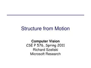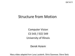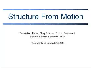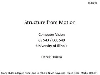
Structure from motion
Structure from motion. Structure from motion. Given a set of corresponding points in two or more images, compute the camera parameters and the 3D point coordinates. ?. ?. Camera 1. ?. Camera 3. ?. Camera 2. R 1 ,t 1. R 3 ,t 3. R 2 ,t 2. Slide credit: Noah Snavely. X j. x 1 j.


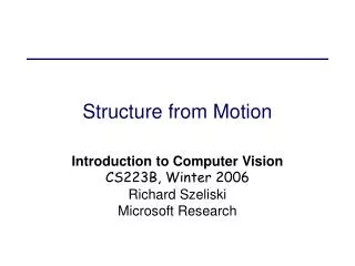
Structure from motion
E N D
Presentation Transcript
Structure from motion • Given a set of corresponding points in two or more images, compute the camera parameters and the 3D point coordinates ? ? Camera 1 ? Camera 3 ? Camera 2 R1,t1 R3,t3 R2,t2 Slide credit: Noah Snavely
Xj x1j x3j x2j P1 P3 P2 Structure from motion • Given: m images of n fixed 3D points • λijxij = Pi Xj , i = 1, … , m, j = 1, … , n • Problem: estimate m projection matrices Piand n 3D points Xjfrom the mn correspondences xij
Is SfM always uniquely solvable? • Necker cube Source: N. Snavely
Structure from motion ambiguity • If we scale the entire scene by some factor k and, at the same time, scale the camera matrices by the factor of 1/k, the projections of the scene points in the image remain exactly the same: • It is impossible to recover the absolute scale of the scene!
Structure from motion ambiguity • If we scale the entire scene by some factor k and, at the same time, scale the camera matrices by the factor of 1/k, the projections of the scene points in the image remain exactly the same • More generally, if we transform the scene using a transformation Q and apply the inverse transformation to the camera matrices, then the images do not change:
Types of ambiguity • With no constraints on the camera calibration matrix or on the scene, we get a projective reconstruction • Need additional information to upgrade the reconstruction to affine, similarity, or Euclidean Projective 15dof Preserves intersection and tangency Preserves parallellism, volume ratios Affine 12dof Similarity 7dof Preserves angles, ratios of length Euclidean 6dof Preserves angles, lengths
Affine ambiguity Affine
Structure from motion • Let’s start with affine or weak perspective cameras(the math is easier) center atinfinity
Recall: Orthographic Projection Image World Projection along the z direction
Affine cameras Orthographic Projection Parallel Projection
x a2 X a1 Affine cameras • A general affine camera combines the effects of an affine transformation of the 3D space, orthographic projection, and an affine transformation of the image: • Affine projection is a linear mapping + translation in non-homogeneous coordinates Projection ofworld origin
Affine structure from motion • Given: m images of n fixed 3D points: • xij = Ai Xj+ bi , i = 1,… , m, j = 1, … , n • Problem: use the mn correspondences xij to estimate m projection matrices Ai and translation vectors bi, and n points Xj • The reconstruction is defined up to an arbitrary affine transformation Q (12 degrees of freedom): • We have 2mn knowns and 8m + 3n unknowns (minus 12 dof for affine ambiguity) • Thus, we must have 2mn >= 8m + 3n – 12 • For two views, we need four point correspondences
Affine structure from motion • Centering: subtract the centroid of the image points in each view • For simplicity, set the origin of the world coordinate system to the centroid of the 3D points • After centering, each normalized 2D point is related to the 3D point Xj by
Affine structure from motion • Let’s create a 2m×n data (measurement) matrix: cameras(2m) points (n) C. Tomasi and T. Kanade. Shape and motion from image streams under orthography: A factorization method.IJCV, 9(2):137-154, November 1992.
Affine structure from motion • Let’s create a 2m×n data (measurement) matrix: points (3× n) cameras(2m ×3) The measurement matrix D = MS must have rank 3! C. Tomasi and T. Kanade. Shape and motion from image streams under orthography: A factorization method.IJCV, 9(2):137-154, November 1992.
Factorizing the measurement matrix Source: M. Hebert
Factorizing the measurement matrix • Singular value decomposition of D: Source: M. Hebert
Factorizing the measurement matrix • Singular value decomposition of D: Source: M. Hebert
Factorizing the measurement matrix • Obtaining a factorization from SVD: Source: M. Hebert
Factorizing the measurement matrix • Obtaining a factorization from SVD: This decomposition minimizes|D-MS|2 Source: M. Hebert
Affine ambiguity • The decomposition is not unique. We get the same D by using any 3×3 matrix C and applying the transformations M → MC, S →C-1S • That is because we have only an affine transformation and we have not enforced any Euclidean constraints (like forcing the image axes to be perpendicular, for example) Source: M. Hebert
Eliminating the affine ambiguity • Transform each projection matrix A to another matrix AC to get orthographic projection • Image axes are perpendicular and scale is 1 • This translates into 3m equations: • (AiC)(AiC)T= Ai(CCT)Ai=Id, i = 1, …, m • Solve for L =CCT • Recover C from L by Cholesky decomposition: L = CCT • Update M and S: M = MC, S = C-1S a1 · a2 = 0 |a1|2 = |a2|2= 1 x AAT= Id a2 X a1 Source: M. Hebert
Reconstruction results C. Tomasi and T. Kanade. Shape and motion from image streams under orthography: A factorization method.IJCV, 9(2):137-154, November 1992.
Algorithm summary • Given: m images and n features xij • For each image i, center the feature coordinates • Construct a 2m ×n measurement matrix D: • Column j contains the projection of point j in all views • Row icontains one coordinate of the projections of all the n points in image i • Factorize D: • Compute SVD: D = U W VT • Create U3 by taking the first 3 columns of U • Create V3 by taking the first 3 columns of V • Create W3 by taking the upper left 3 × 3 block ofW • Create the motion and shape matrices: • M = U3W3½ and S = W3½V3T(or M = U3 and S = W3V3T) • Eliminate affine ambiguity Source: M. Hebert
Dealing with missing data • So far, we have assumed that all points are visible in all views • In reality, the measurement matrix typically looks something like this: cameras points
Dealing with missing data • Possible solution: decompose matrix into dense sub-blocks, factorize each sub-block, and fuse the results • Finding dense maximal sub-blocks of the matrix is NP-complete (equivalent to finding maximal cliques in a graph) • Incremental bilinear refinement • Perform factorization on a dense sub-block (2) Solve for a new 3D point visible by at least two known cameras (linear least squares) (3) Solve for a new camera that sees at least three known 3D points (linear least squares) F. Rothganger, S. Lazebnik, C. Schmid, and J. Ponce. Segmenting, Modeling, and Matching Video Clips Containing Multiple Moving Objects. PAMI 2007.
Xj x1j x3j x2j P1 P3 P2 Projective structure from motion • Given: m images of n fixed 3D points • λijxij = Pi Xj, i = 1,… , m, j = 1, … , n • Problem: estimate m projection matrices Pi and n 3D points Xj from the mn correspondences xij
Projective structure from motion • Given: m images of n fixed 3D points • λijxij = Pi Xj, i = 1,… , m, j = 1, … , n • Problem: estimate m projection matrices Pi and n 3D points Xj from the mn correspondences xij • With no calibration info, cameras and points can only be recovered up to a 4x4 projective transformation Q: • X → QX, P → PQ-1 • We can solve for structure and motion when • 2mn >= 11m +3n – 15 • For two cameras, at least 7 points are needed
Projective SFM: Two-camera case • Compute fundamental matrixF between the two views • First camera matrix: [I | 0] • Second camera matrix: [A | b] • Then b is the epipole (FTb= 0), A = –[b×]F F&P sec. 8.3.2
Sequential structure from motion • Initialize motion from two images using fundamental matrix • Initialize structure by triangulation • For each additional view: • Determine projection matrix of new camera using all the known 3D points that are visible in its image – calibration points cameras
Sequential structure from motion • Initialize motion from two images using fundamental matrix • Initialize structure by triangulation • For each additional view: • Determine projection matrix of new camera using all the known 3D points that are visible in its image – calibration • Refine and extend structure: compute new 3D points, re-optimize existing points that are also seen by this camera – triangulation points cameras
Sequential structure from motion • Initialize motion from two images using fundamental matrix • Initialize structure by triangulation • For each additional view: • Determine projection matrix of new camera using all the known 3D points that are visible in its image – calibration • Refine and extend structure: compute new 3D points, re-optimize existing points that are also seen by this camera – triangulation • Refine structure and motion: bundle adjustment points cameras
Bundle adjustment • Non-linear method for refining structure and motion • Minimizing reprojection error Xj P1Xj x3j x1j P3Xj P2Xj x2j P1 P3 P2
Modern SFM pipeline N. Snavely, S. Seitz, and R. Szeliski, "Photo tourism: Exploring photo collections in 3D," SIGGRAPH 2006.
Feature detection • Detect features using SIFT [Lowe, IJCV 2004] Source: N. Snavely
Feature detection Detect features using SIFT [Lowe, IJCV 2004] Source: N. Snavely
Feature matching Match features between each pair of images Source: N. Snavely
Feature matching Use RANSAC to estimate fundamental matrix between each pair Source: N. Snavely
Image connectivity graph (graph layout produced using the Graphviz toolkit: http://www.graphviz.org/) Source: N. Snavely
Incremental SFM • Pick a pair of images with lots of inliers (and preferably, good EXIF data) • Initialize intrinsic parameters (focal length, principal point) from EXIF • Estimate extrinsic parameters (Rand t) • Five-point algorithm • Use triangulation to initialize model points • While remaining images exist • Find an image with many feature matches with images in the model • Run RANSAC on feature matches to register new image to model • Triangulate new points • Perform bundle adjustment to re-optimize everything
The devil is in the details • Handling degenerate configurations (e.g., homographies) • Eliminating outliers • Dealing with repetitions and symmetries • Handling multiple connected components • Closing loops • ….
Review: Structure from motion • Ambiguity • Affine structure from motion • Factorization • Dealing with missing data • Incremental structure from motion • Projective structure from motion • Bundle adjustment • Modern structure from motion pipeline
Summary: 3D geometric vision • Single-view geometry • The pinhole camera model • Variation: orthographic projection • The perspective projection matrix • Intrinsic and extrinsic parameters • Calibration • Single-view metrology, calibration using vanishing points • Multiple-view geometry • Triangulation • The epipolar constraint • Essential matrix and fundamental matrix • Stereo • Binocular, multi-view • Structure from motion • Reconstruction ambiguity • Affine SFM • Projective SFM