
Understanding Isoquants and Constant Returns to Scale in Production Theory
This text explores the concept of isoquants in the context of constant returns to scale. It illustrates how a proportional increase in inputs, such as labor and capital, will lead to an equivalent proportional increase in output. By analyzing points on the isoquants, we demonstrate that if cost minimization is achieved at one level of output, it will also be maintained at different levels. The radial nature of isoquants simplifies cost minimization, as knowing the ideal input mix for one output level allows easy calculations for other levels.

Understanding Isoquants and Constant Returns to Scale in Production Theory
E N D
Presentation Transcript
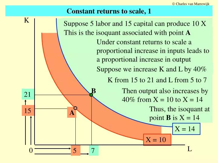
Charles van Marrewijk K B 21 15 A X = 14 X = 10 L 0 5 7 Constant returns to scale, 1 Suppose 5 labor and 15 capital can produce 10 X This is the isoquant associated with point A Under constant returns to scale a proportional increase in inputs leads to a proportional increase in output Suppose we increase K and L by 40% K from 15 to 21 and L from 5 to 7 Then output also increases by 40% from X = 10 to X = 14 Thus, the isoquant at point B is X = 14
Charles van Marrewijk K But if A’ is another point on the X=10 isoquant we can use the same procedure to conclude that B’ must be also on the X=14 isoquant B’ 44 B A’ 40 110 A 100 X = 14 X = 10 L 0 Constant returns to scale, 2 Increasing the inputs at A with 40% is equivalent to increasing the length of a line from the origin through A with 40% This procedure can be repeated for any arbitrary point on the X=10 isoquant; here are a few The X = 14 isoquant is a blow-up radial
Charles van Marrewijk K B 21 A 15 X = 14 X = 10 L 0 5 7 Constant returns to scale, 3 Under constant returns to scale the isoquants are radial blow-ups of each other, which implies that drawing 1 isoquant gives information on all others For example, that if cost is minized at point A for X = 10, then it is also minimized at the 40% radial blow-up of A (B) for X = 14 Thus, the slope of the isoquant at point A is the same as at point B
Charles van Marrewijk K B 21 A 15 X = 14 X = 10 L 0 5 7 Constant returns to scale, 4 Since the isoquants are radial blow-ups of one another and the slope at point A is the same as the slope at point B cost minimization is simpler. If we know the cost minimizing input mix for one isoquant and any ratio of w/r, we also know it for any other production level. You only have to multiply the input mix times the output ratio (we frequently use the isoquant X = 1)