Download
1 / 21
210 likes | 355 Vues
Assimilating radiances from polar-orbiting satellites in the COSMO model by nudging. Reinhold Hess , Detlev Majewski Deutscher Wetterdienst. Specific issues of limited area models for the use of satellite data (radiances). assimilation scheme

E N D
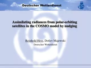
Assimilating radiances from polar-orbiting satellites in the COSMO model by nudging Reinhold Hess, Detlev Majewski Deutscher Wetterdienst
Specific issues of limited area models for the use of satellite data (radiances) • assimilation scheme • provide initial value fit and consistent with the limited area model • use temporally and spatially highly resolved observations • (background and observations errors and correlations) • complex and situation dependent statistics for background and observation errors, flow dependence, more critical vertical structure (temp/hum/wind) • bias correction • sample size, representativity of samples, overfitting, choice of predictors • first guess above model top • tuning of observations (thinning) • use of data over land (surface emissivity, higher resolution of surface conditions) • verification • statistical representativity of results, influence of boundary values
xb 9 6 0 3 Nudging approach (Newtonian Relaxation Scheme): The model trajectory is nudged in every time step towards the observations with special terms additional to the model dynamics (nudging towards observations during forecast). The sizes of the terms depend on the distance to the observations and on the time difference between observation and current model time. Difficult to use nonlinear observations analysis at time ta initial time t0 yo Model trajectory relaxed toward observations model state xa Allobservations yo are used mainly at their actual time but also before and after 12 time assimilation window
Temporal Weighting (for frequent data: linear interpolation) Use of nonlinear operators with nudging at appropriate time Conventional observations: nudge observation 1.5 h before (and 30 min after) observation time with temporal weighting depending on time difference to observation Satellite data: 1D-Var preliminary retrievals of temperature and humidity have to be computed. For nonlinear observations use first guess available -1.5 h before observation time. Repeat retrieval every 30 min until nudging analysis reaches observation time. Attention: first guess and observation become correlated!
HOURS 12 12 12 12 12 00 00 00 00 00 time 1 2 3 4 5 6 DAYS Error covariance matrix B The B matrix is calculated using forecast comparisons at +12h and +36h averaged over three months. Hour of comparison of the two forecasts
Background error covariance matrix B complication: error structures from lateral boundary values • standard NMC-method • (large error structures in statistics do not reflect small scale errors) • lagged NMC-method (ALADIN): use identical boundary values • (use boundary values from the same run of the embedding model) • no boundary errors lead to error statistics of smaller scale • ensemble B: pertubated observations or physics • error statistics somehow in between standard and lagged NMC-method • However: • less constraints on B (geostrophy, hydrostacy) • high variation in error structures, more motivation for weather • situation dependent, flow dependent or adaptive error structures
for given error variance the required sample size is examples: for Bias Correction for ATOVS scanline and airs mass dependent correction (Eyre, Harris & Kelly) scanline correction: what is reasonable sampling size? • variance of a mean variable is • application to obs – fg brightness temperatures: (statistics are for each individual fov) • time to obtain required sample sizes for individual fovs depend on model area (size over sea) • for COSMO-EU two weeks for most relevant temperature sounding channels • what about representativity (synoptic scenarious, seasonal changes) ?
scanline biases AMSU/NOAA 18 (15 to 25 June 2007) GME lat 30 to 60 deg, lon:-30 to 0 deg COSMO-EU: approx 1200-1500 fovs approx 1200 obs/fov approx 1000-1500 obs/fov
scanline biases AMSU/NOAA 18 (15 to 25 June 2007) GME lat 30 to 60 deg, lon:-30 to 0 deg COSMO-EU: approx 1200-1500 fovs lapse rate? approx 1200 obs/fov approx 1000-1500 obs/fov
Bias Correction for ATOVS scanline correction • irregular shape • constant with area (for most channels, no lattitude dependency) • sample size not too critical • representativity seems no issue • GME and COSMO-EU show significant differences only for surface • (and humidity channels) • no significant influence of interpolation with ATOVPP/AAPP • (6 resp. 4 side fovs removed) air mass correction • idea: air mass bias is situation dependent, model these biases using meteorological predictors • choices of predictors: • AMSU-A 5 and 9 (observed or simulated) • mean temperatures (50-200 hPa and 300-1000 hPa), SST, IWV • predictors for scanline correction: zenith angle, square of zenith angle (or remove scanline correction before air mass correction) • latitude as predictor/coefficients variable with latitude band What is a good choice of predictors?
Time series of bias corrected observations minus first guess AMSU-A channels 4-11, NOAA-18 stable in the troposphere, however large variations for high sounding channels
Provide first guess values above model top Limited area models usually have lower model top than required by RTTOV (0.1hPa - 0.05hPa) COSMO-EU: 30hPa HIRLAM: 10hPa ALADIN: 1hPa • increase height of model top • use climatological values (inaccurate, use only lower peaking channels) • use forecasts of global model IFS (accurate, but timely receive of IFS forecasts required) • linear regression of high peaking channels to model levels (Met Office) y = W x x: high peaking channels y: temperatures on RTTOV levels W: regression matrix compute W with training data set • reasonable: • no humidity • more or less linear relation between, high peaking channels and level temperature • (no clouds)
Provide first guess values above model top (COSMO-EU: 30hPa) • use of climatological values (ERA40) seems not sufficient • linear regression of top RTTOV levels from stratospheric channels • (other choice: use IFS forecasts as stratospheric first guess) ECMWF profiles versus estimated profiles, top GME levels accuracy about 5K for lower levels, but ECMWF may have errors in stratosphere, too levels: 0.10, 0.29, 0.69, 1.42, 2.611, 4.407, 6.95, 10.37, 14.81 hPa
1D-Var for COSMO-EU: Cloud and Rain detection Microwave surface emissivity model: rain and cloud detection (Kelly & Bauer) Validation with MSG imaging Validation with radar data
T-‘analysis increments’ from ATOVS, after 30 minutes (sat only), k = 20 no thinning of 298 ATOVS 30 ATOVS by old thinning (3) 30 ATOVS, correl. scale 70% 40 ATOVS by thinning (3) 82 ATOVS by thinning (2) 82 ATOVS, correl. scale 70%
mean sea level pressure & max. 10-m wind gusts valid for 20 March 2007 , 00 UTC m/s + 48 h, REF (no 1D-VAR) analysis + 48 h, 1D-VAR-THIN3 + 48 h, 1D-VAR-THIN2
Forecast quality of regional models depend on ... • initial state • fit to observations (truth) • consistency with numerical model, small scale features in initial state (resolution, orography, vertical distribution of humidity, etc.) • numerical model, resolution, approximations (e.g. hydrostacy), • physics (e.g. convection), parameterisations • quality of boundary values • timeliness of forecast, (short range forecasting) Limited area models ... • high resolution (2 - 20 km) • small scale structures in space and time (e.g. convection) • delicate physics (e.g. steep orography, discontinuous solutions, bifurcations) • limited predictability of small scale phenomena (computationally and physically) • fewer constraints (e.g. hydrostacy, geostrophy) • need to use asynchronous and high frequent observations (e.g. SEVIRI/MSG, radar) • limited area (driven by lateral boundary values of coarser scale models) • over land (use of radiances over land)
xa xb 3 6 9 4D-Var approach: initial state minimises misfits of model trajectory to observations and deviation from first guess. 3D-Var: as 4D-Var, but all observations valid for time of analysis, no computation of trajectory during minimisation 3D-Var-FGAT: use trajectory at observation time for first guess, but keep innovations constant All information has to be reflected in initial state (analysis) model state Allobservations yo between ta-9h and ta+3h are used at their actual time (3D-Var) analysis at time ta initial time t0 yo Model trajectory from analysed initial state xa Model trajectory from first-guess xb (= model background state) 12 15 time 4D-Var assimilation window
Pros and Cons for limited area models 4D-Var: + use of asynchronous observations + nonlinear observations can be used + consistent mathematical framework (obs and fg errors) - solutions are less smooth and predictable (physically) - physics are more complex (tangent linear and adjoint) - specification of background errors is more difficult (boundary, fewer constraints) - time consuming 3D-Var (EnKF): + consistent mathematical framework + combination with ensemble methods - use of observations at time of analysis - requires initialisation Nudging: + unsteady solutions, complicated physics + use of anynchronous and high frequent observations + fast, provide timely forecast + no initialisation required + combination with ensemble methods - use of nonlinear observation operators - no consistent mathematical framework, lots of tuning required