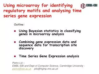
Using microarray for identifying regulatory motifs and analysing time series gene expression

1. Using microarray for identifying regulatory motifs and analysing time series gene expression Outline: • Using Bayesian statistics in classifying genes in microarray analysis • Combining gene expression data and sequence data for transcription site discovery • Time Series Gene Expression analysis Pietro Lió – EMBL-EBI and Dept of Computer Science, Cambridge University - pietrol@ebi.ac.uk plio@hgmp.mrc.ac.uk

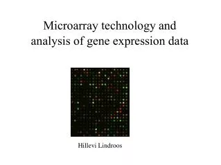
2. Types of questions What genes are expressed in a particular cell type of an organism, at a particular time, under particular conditions? Comparison of gene expression between normal and diseased (e.g., cancerous) cells.

3. A typical dimension of such an array is about 1 inch or less. • The spot diameter is of the order of 0.1 mm, for some microarray types can be even smaller. 

4. One of the most popular microarray applications allows to compare gene expression levels in two different samples, e.g., the same cell type in a healthy and diseased state.

5. Classification of genes in microarray analysis • Microarray statistics can be supervised or unsupervised. • In the unsupervised case, only the expression data are available and the goal is mainly to identify distinct sets of genes with similar expressions, suggesting that they may be biologically related. • In supervised problems a response measurement is also available for each sample and the goal of the experiment is to find sets of genes that, for example, relate to different kind of diseases, so that future tissue samples can be correctly classified.

6. Bayesian Statistics • Bayesian statistics models all source of uncertainty (physical randomness, subjective opinions, prior ignorance, etc) with probability distributions and then trying to find the a posteriori distribution of all unknown variable of interest after considering the data. Bayes, T. 1763. An essay towards solving a problem in the doctrine of chances. Philosophical Transactions of the Royal Society of London 53:370-418. Reprinted, E. S. Pearson and M. G. Kendall (eds.). 1970. Pages 131-153 in Studies in the History of Statistics and Probability. Charles Griffin, London.

7. In Bayesian statistics, evidences in favour of certain parameter θ is considered: Inference is based on posterior distribution, Pr(θ|D) which is the conditional distribution of the parameter given the data, D. It is a combination of the prior information and the data. The term Pr(θ) represents the prior distribution on the parameter. Prior information can be based on previous experiments, or theoretical consideration. The term Pr(D|θ) can be a likelihood and the denominator Pr(D) is a normalizing factor.

8. First write down the likelihood function, i.e. the probability of the observed data given the unknowns, and multiply it by the a priori distribution. • Let D denote the observed data and θ the unobserved parameter. • Through the application of the Bayes theorem we can obtain the posterior distribution: Whenθis discrete, the integral is replaced by summation.

9. Bayesian Learning Posterior is prior modified by data Flat (“uninformative prior”) 1 0 θ

10. MCMC The most useful method to approximate the posterior probability is Monte CarloMarkov chain (MCMC). MCMC, ……. …consider a robot random walking in a landscape with hills…(these hills will be the genes involved in a disease or a set of regulatory regions but you will see later) Imagine a bivariate normal hills and the Markov chain represents the positions of steps taken by a robot.

11. A proposed move is always accepted if it is “uphill” and is often accepted if it is not too much “downhill” from the current position. hills RULE: The step would be rejected if the elevation at proposed new location is less than that of the current location, and the uniform random number drawn was greater than the ratio of new elevation to old elevation.

12. The inner and the outer circles represent 50% and 95% probability contours for the bivariate normal density The robot visits points in proportion to their height. Since the height represents the value of the probability density function, we can simply count the dots in order to obtain an approximation of the probability corresponding to a given area. In other words, the necessary integration of the density function is approximated by the MCMC run. BURN IN: the initial steps (the “burn in”) are often discarded in a MCMC run.

13. A proposed move is always accepted if it is “uphill” and is often accepted if it is not too much “downhill” from the current position. • Formally, in the Metropolis-Hastings (Metrolis et al., 1953, Hastings, 1970) algorithm, a move from θ to θ* is accepted with probability min(r,1), where Longer runs of the chain result in better approximations to posterior probabilities, and stopping too soon can have serious consequences (chain may not have been visited large portions of the parameters space).

14. Below is a plot showing the natural logaritm of the posterior probability density (i.e. the elevation) for each point visited by the robot. These are often called “history plots” . Plots like this are often made for MCMC runs to see how well the chain is “mixing”.

15. Mixing and MCMCMC Setting the step size too small runs the risk of missing the big picture: the robot may explore one hill in the landscape very well but not take steps large enough to ever traverse the gap between hills.

16. MCMCMC (MC)3 The solution is to run several Markov chains simultaneously, letting one of them (the “cold”) chain to be the one that counts, and the others (called “the heated” chains) serve as scouts for the cold chain.

17. Data set on Golub et al. (Science 286, 531-537, 1999) on cancer classification that has 38 samples and expression profiles of thousands of genes. Samples are classified into acute lymphoblastic and acute myeloid leukemia. 34 further samples available for validation. • Data set of Alon et al. (PNAS 96, 6745-6750,1999) on colon cancer classification that has a total of 62 samples and expression profiles of 2000 genes.

18. The method is based on using a regression setting and a Bayesian priors to identify the important genes. • The model assigns a prior probability to all possible subsets of genes and then proceeds by searching for those subsets that have high posterior probability. • This method is able to locate small sets of genes that lead to a good classification results.

19. MCMC and microarray The MCMC involves 2 steps: • (i) A subset of genes is proposed by stochastically adding or dropping one gene each time. • (ii) This set is then either accepted or rejected with a probability described by Metropolis and Hastings . • If a new set is accepted, then it is subjected to further perturbation.

20. Output: set of genes that differ among the two types of leukemia genes Leukemia classification: posterior probabilities for single genes in 9 runs

21. Leukemia classification: renormalized posterior probabilities for single genes

23. Some results from leukemia data set • Cystatin A and C belong to cystein protease inhibitors. Cystein proteases induce apoptosis of leukemia cells. • IL-8 is a chemokine released in response to an inflammatory stimulus that attracts and activates several types of leukocytes. IL-8 gene is close to several other genes involved in cancer, such as the interferon gamma induced factor. • Adipsin (Complement factor D) is a serine protease secreted by adipocytes involved in antibacterial host defense. Note that IL-8 is also released from human adipose tissue. • Zyxin is a LIM-domain protein localized in focal cell- adhesion.

25. Some results from Colon cancer data set • CRP contains 2 copies of LIM domain (acting cell growth factors); its expression is parallel to that of c-myc that has an abnormally high expression in a wide variety of human tumours. It interacts with cytoskeleton and cell- adhesion proteins. • Myosin regulatory light chain 2 binds calcium ions and regulate contractile activity of several cell types. It is present in several EST cDNA extracted from a large number of tumours.

26. Regulatory regions discovery using gene expression data Related to Reverse engineering of genetic networks • Related genes that have similar expression profiles are likely to have similar regulation mechanisms as there must be a reason why their expression is similar under a variety of conditions (not always true!). • If we cluster the genes by similarities in their expression profiles and take sets of promoter sequences from genes in such clusters, some of these sets of sequences may contain a ‘pattern’ which is relevant to regulation of these genes

27. Combining sequence and gene expression data to find transcription sites The search for transcription sites often starts from the assessment of the statistical significance of over- or under-representation of oligomers in complete genomes that may indicate phenomena of positive or negative selection.

28. 5’- TCTCTCTCCACGGCTAATTAGGTGATCATGAAAAAATGAAAAATTCATGAGAAAAGAGTCAGACATCGAAACATACAT …gene1 …gene2 5’- ATGGCAGAATCACTTTAAAACGTGGCCCCACCCGCTGCACCCTGTGCATTTTGTACGTTACTGCGAAATGACTCAACG 5’- CACATCCAACGAATCACCTCACCGTTATCGTGACTCACTTTCTTTCGCATCGCCGAAGTGCCATAAAAAATATTTTTT …gene3 5’- TGCGAACAAAAGAGTCATTACAACGAGGAAATAGAAGAAAATGAAAAATTTTCGACAAAATGTATAGTCATTTCTATC …gene4 …gene5 5’- ACAAAGGTACCTTCCTGGCCAATCTCACAGATTTAATATAGTAAATTGTCATGCATATGACTCATCCCGAACATGAAA 5’- ATTGATTGACTCATTTTCCTCTGACTACTACCAGTTCAAAATGTTAGAGAAAAATAGAAAAGCAGAAAAAATAAATAA …gene6 5’- GGCGCCACAGTCCGCGTTTGGTTATCCGGCTGACTCATTCTGACTCTTTTTTGGAAAGTGTGGCATGTGCTTCACACA …gene7 AAAAGAGTCA AAATGACTCA AAGTGAGTCA AAAAGAGTCA GGATGAGTCA AAATGAGTCA GAATGAGTCA AAAAGAGTCA ********** Finding the sequences (protein binding sites) that affect the gene expression

29. Motif Gene expression

30. Strategy diagram • Rank all genes by expression and obtain their upstream sequences • Find motifs from promoters of most induced and most repressed genes • Score each upstream sequence for matches to each considered motif • Perform variable selection on the significant motifs to find group of motifs acting together to affect expression

31. MCMC and microarray The MCMC involves 2 steps: • A new subset of motifs is proposed by stochastically adding or dropping one motif each time. • This set is then either accepted or rejected with a probability described by Metropolis and Hastings .

32. Gene expression data, combined with sequence analysis, seem to represent a promising method to identify transcription sites. • We consider both yeast sequences and expression data and outputs statistically significant motifs: the regions upstream genes contribute to the log-expression level of a gene. • First we have first identified a number of sequence patterns upstream the yeast genes and then tested for candidate transcription sites.

35. Finding all cell-cycle genes from gene expression data Periodically expressed genes Intensity Non periodically expressed genes Time measure

36. Cell-cycle experiments

37. J.B. Fourier (1768-1830) time frequency

39. Regression using Fourier terms Suppose Yi(t) denotes the expression of gene i at time t. For all genes the vector Yi(t) was fit first with least squares to Yi(t)=aiS(t)+biC(t)+Ri(t), where S(t)=sin(2pt/T) and C(t)=cos(2pt/T) with T is the period of the cell cycle. Yi(t) can be decomposed into a periodic component Zi(t)=aiSi(t)+biCi(t) and a component Ri(t) that is aperiodic.

40. The proportion of variance explained by the Fourier basis (Fourier proportion of variance explained -PVE) is the ratio mi=var(Zi(t))/var(Yi(t)), which can range from 0 to 1. Values closer to 1 indicate greater sinusoidal expression, whereas values closer to 0 indicate lack of periodicity or periodicity with a period that is substancially different. The fitted waveform Z(t) resembles a sine wave. For each gene, the phase of Z(t) (equal to time of maximal expression) was determined.

43. Wavelets • A wavelet is an oscillation that decays quickly • are related to fractals in that the same shapes repeat at different orders of magnitude. • outperforms a Fourier when the signal under consideration contains discontinuities and sharp spikes • differ from Fourier methods in that they allow the localization of a signal in both time and frequency

44.  A wavelet is an oscillation that decays quickly Wavelet basis are related to fractals in that the same shapes repeat at different orders of magnitude A function can be represented in wavelet domain by the an infinite series expansion of dilated and translated version of a function : J, scale parameter K, position parameter Each wavelet function jkis multiplied by a wavelet coefficient

45. Wavelet methods differ from Fourier methods in that they allow the localization of a signal in both time and frequency Fourier Local Fourier Wavelet transform the time/frequency plane is patched with rectangles of different shape w w w t t t When modeling time/frequency phenomena no precision in time and frequency at the same time! f(t) w w Instant frequency Impossible! t t t

46. Wavelet coefficients: the upper ones describe gross features of the signal, the bottom ones descrive little details Scale J Position,k Denoising and extraction of components of figure a The sum of the squares of the wavelet coefficients at each scale is termed a scalogram

47. Periodic Analysis of single time series The wavelet variance of periodically expressed genes is 100 times larger than that of non periodic genes

48. Non Periodic Confidence intervals wavelet variance is a scale by scale decomposition of the variance of a signal. Replacing ‘global’ variability with variability over scales allows us to investigate the effects of constraints acting at different time or sequence-length scales

49. Cell cycle analysis Errors for Anova in time domain Reconstruction by an Anova in time domain Reconstruction by an Anova in wavelet domain Errors for Anova in wavelet domain RESULTS: Residual errors are smaller in wavelet domain -> BETTER ESTIMATE OF VARIANCE USING WAVELETS

50. FDR false discovery rate Bonferroni method belongs to a class of methods called family-wise type I error rate (FWE), which is the probability of committing at least one error in the family of hypotheses. The main problem with classical procedures, such the Bonferroni correction, which hinder many applications in biology, is that they tend to have substantially less power than uncorrected procedures. Recent FEW methods have been used in microarray by Dudoit et al (2002) The multiplicity problem in microarray data does not require a protection against even a single type I error, so that the severe loss of power involved in such protection is not justified. Instead, it may be more appropriate to emphasize the proportion of errors among the identified differentially expressed genes. The expectation of this proportion is the False Discovery Rate (FDR) of Benjamini and Hochberg (1995). The FDR is the expected proportion of true null hypotheses rejected out of the total number of null hypotheses rejected.