Download
1 / 12
120 likes | 298 Vues
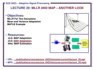
LECTURE 20: MLLR AND MAP – ANOTHER LOOK. Objectives: MLLR For Two Gaussians Mean and Variance Adaptation MATLB Example Resources: JLG: MAP Adaptation JLG: MAP Adaptation Wiki: MAP Estimation. • URL: .../publications/courses/ece_8423/lectures/current/lecture_20.ppt

E N D
LECTURE 20: MLLR AND MAP – ANOTHER LOOK • Objectives:MLLR For Two GaussiansMean and Variance AdaptationMATLB Example • Resources:JLG: MAP AdaptationJLG: MAP AdaptationWiki: MAP Estimation • URL: .../publications/courses/ece_8423/lectures/current/lecture_20.ppt • MP3: .../publications/courses/ece_8423/lectures/current/lecture_20.mp3
MLLR Example (Revisited) • Let us consider the problem of the adaptation of the parameters associated with two Gaussians: • We choose to adapt the mean parameters using an affine transformation (essentially a regression model): • Since this is a single dimension Gaussian, the variance will simply be scaled: • Our goal is to estimate the transformation parameters: • We would like to do this using N points of training data (old data) and M points of adaptation data (new data), where typically N >> M. • The solution we seek will essentially replace the mean of the old data with the mean of the new data, but it will do this through estimation of a transformation matrix rather than simply using the sample mean.
Establishing an Auxiliary Function • The latter (reestimation by using the sample mean), we will soon see, can be regarded as a variant of a maximum a posteriori estimate. The drawback of this approach is two-fold: • Reestimation using the sample mean requires the state or event associated with that Gaussian to be observed. In many applications, only a small percentage the events associated with specific Gaussians are observed in a small adaptation set. The transformation matrix approach allows us to share transformation matrices across states, and hence adapt the parameters associated with unseen events or states. • Through transformation sharing, we can intelligently, based on the overall likelihood of the data given the model, cluster and share parameters, and to do this in a data-driven manner. This is extremely powerful and gives much better performance than static or a priori clustering. • Assume a series of T observations, , where oi is simply a scalar value that could have been generated from one of two Gaussians. • Define an auxiliary Q-function for parameter reestimation based on the EM theorem such that its maximization will produce an ML estimate:
Establishing an Auxiliary Function • This auxiliary function is simply the total likelihood. There are T observations, each of which could have been produced by one Gaussian. Hence, there are four possible permutations, and this function sums the “entropy” contribution of each outcome. • However, note that we use both the current model, , and the new, or adapted model, , in this calculation, which makes it resemble a divergence or cross-entropy. This is crucial because we want the new model to be more probable given the data than the old model. • Recall two simple but important properties of conditional probabilities: • The latter is known as Bayes’ Rule. • Applying these to the likelihood in our auxiliary function: • Also, we can expand the log:
Minimizing the Auxiliary Function • Therefore, we can write our auxiliary function as: • We can differentiate w.r.t. our transformation coefficients, wi,j, and set to 0: • Solve for the new mean:
Mean Adaptation • This is an underdetermined system of equations – one equation and two unknowns. • Use a pseudoinverse solution which adds an additional constraint that the parameter vector should have the minimum norm. Use “+” to denote this solution: • This pseudoinverse is found using singular value decomposition. In this case this returns the weight vector that has a minimum norm. • Note that if each Gaussian is equally likely, then the computation reduces to the sample mean.
Variance Adaptation: • Recall our expression for the auxiliary function • Recall also that: • We can differentiate Q with respect to si: • Equating this to zero gives the ML solution: • Hence:
Example (MATLAB Code) clear; N=500; M=200; mu_train=2.0; var_train=1.0; x_train=mu_train+randn(1,N)*sqrt(var_train); mu_test=2.5; var_test=1.5; x_test=mu_test+randn(1,M)*sqrt(var_test); mean_hat=[]; var_hat=[]; for i=1:M m=mean(x_test(1:i)); w = pinv([1 mu_train])*m; mean_hat=[mean_hat [1 mu_train]*w]; v=var(x_test(1:i)); s=v/var_train; var_hat=[var_hat s*var_train]; end; subplot(211);line([1,M],[mu_train, mu_train],'linestyle','-.'); hold on; subplot(211);line([1,M],[m, m],'linestyle','-.','color','r'); subplot(211);plot(mean_hat); text(-32, mu_train, 'train \mu'); text(-32, m, 'adapt \mu'); title('Mean Adaptation Convergence'); subplot(212);line([1,M],[var_train, var_train],'linestyle','-.'); hold on; subplot(212);line([1,M],[v, v],'linestyle','-.','color','r'); subplot(212);plot(var_hat); text(-32, var_train, 'train \sigma^2'); text(-32, v, 'adapt \sigma^2'); title('Variance Adaptation Convergence');
Maximum A Posteriori (MAP) Estimation • Suppose we are given a set of M samples from a discrete random variable, x(n), for n=0,1,…,M-1, and we need to estimate a parameter, , from this data. • We assume the parameter is characterized by a probability density function, f(), that is called the a priori density. • The probability density function f(|x) is the probability density of conditioned on the observed data, x, and is referred to as the a posteriori density for . • The Maximum A Posteriori (MAP) estimate of is the peak value of this density. • The maximum can generally be found by: . We refer to the value of that maximizes this equation as MAP . • We often maximize the log of the posterior: . • Determination of f(|x) is difficult. However, we use Bayes’ rule to write: • where is the prior density of . • Applying a logarithm, we can write theMAP solution as:
Summary • Demonstrated MLLR on a simple example involving mean and variance estimation for two Gaussians. • Reviewed a MATLAB implementation and MATLAB simulation results.