Download
1 / 20
200 likes | 230 Vues
Learn the methods (FEM, BEM, FVM, FD) & requirements (consistency, stability, conservativeness) of CFD solvers for accurate simulations and results in complex systems. Understand the importance of approximation, stability, and boundedness for numerical schemes.

E N D
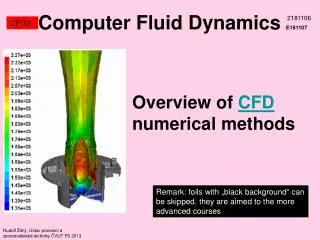
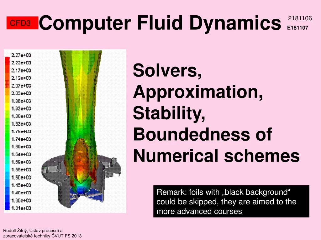
ComputerFluid DynamicsE181107 2181106 CFD3 Solvers,Approximation, Stability, Boundedness of Numerical schemes Remark: foils with „black background“ could be skipped, they are aimed to the more advanced courses Rudolf Žitný, Ústav procesní a zpracovatelské techniky ČVUT FS 2013
SOLVERS CFD3 • FEM, BEM, FVM, FD transfer PDE into system of algebraic equations for Tj (nodal pressures, velocities, temperature, concentrations…) solved by • Finite methods (Gauss, SVD, LU decomposition, frontal methods) N3 operations are required – suitable for smaller systems. • Iterative methods (GS, multigrid, GMRES, conjugated gradients). Prevails at CFD calculations, characterized by number cells (nodes) of several millions and parallel processing (external as well as internal aerodynamics of cars requires up to 108 finite volumes, solved in clusters of e.g. 512 and more processors) Iterative methods are not so sensitive to round-off errors (that’s why they can be applied for such huge systems) Rudolf Žitný, Ústav procesní a zpracovatelské techniky ČVUT FS 2010
Mathematical Requirements CFD3 • Three Mathematical requirements • consistency (discretized equation for must be identical with PDE) order of accuracy (m-with respect time, n-with respect to spatial approximation) • stability (attenuation of round-off errors or glitches of initial conditions) • convergency. Lax theorem: consistent and stable numerical scheme converges to exact solution (but it holds only for linear systems) Rudolf Žitný, Ústav procesní a zpracovatelské techniky ČVUT FS 2010
Physical Requirements CFD3 • Three Physical requirements • Conservativeness. Balance of mass should hold exactly at an element level and globally. Fulfilled by FVM (Finite Volume Method). Not exactly satisfied fy FEM. • Boundedness. Solution should not exhibit local min/max in the absence of internal sources (of mass, momentum or heat). Solution should be bounded by boundary values. Min/max principle. • Transportivness. Numerical scheme should reflect directionality of information transfer (convection along streamlines) Rudolf Žitný, Ústav procesní a zpracovatelské techniky ČVUT FS 2010
Numerical method-analysis CFD3 Few examples, how to analyze order of accuracy and stability of suggested numerical schemes (FD methods) Benton Rudolf Žitný, Ústav procesní a zpracovatelské techniky ČVUT FS 2013
Ti-1 Ti Ti+1 x Order of accuracy CFD3 Taylor expansion Approximation of first derivative Higher Order Terms Accurate for 2nd order polynomialsT=1,x,x2 = Accurate for 1nd order polynomialsT=1,x = Approximation of second derivative Accurate for 3rd order polynomialsT=1,x,x2,x3 = Rudolf Žitný, Ústav procesní a zpracovatelské techniky ČVUT FS 2010
Ti-1 Ti Ti+1 x Order of accuracy CFD3 • Therefore finite differences substituting derivatives at node xi are • First order • Second order • Third order Rudolf Žitný, Ústav procesní a zpracovatelské techniky ČVUT FS 2010
n+1 ∆t n j-1 j ∆x j+1 Stability example (explicit method) CFD3 Unsteady heat transfer (Fourier equation – parabolic) T-temperature, a-temperature diffusivity Finite difference method EXPLICIT (explicit means that unknown temperatures at a new time level can be expressed explicitly, without necessity to solve a system of algebraic equations). What is the order of accuracy? Rudolf Žitný, Ústav procesní a zpracovatelské techniky ČVUT FS 2010
n+1 ∆t n j-1 j ∆x j+1 Stability example (explicit method) CFD3 Residual of this PDE is therefore Scheme is consistent, linear with respect time, cubic with respect space. Rudolf Žitný, Ústav procesní a zpracovatelské techniky ČVUT FS 2010
Stability example (explicit method) CFD3 Rewrite the explicit formula to the following (explicit) form Unknown temperature at a new time level Known temperatures at “old” time level • Rules: • Sum of coefficients must be the same on the left and on the right side (1=A+A+1-2A). Why? A constant solution must be fulfilled exactly! • All coefficients must be positive for bounded solution. Why? • Scarborough criterion (sum of absolute values of off-diagonal elements diagonal element, criterion for convergency of iterative methods) Rudolf Žitný, Ústav procesní a zpracovatelské techniky ČVUT FS 2010
Stability example (explicit method) CFD3 So why all coefficients must be positive for bounded solution? Resulting value T is calculated as a weighted average of values (sum of weighting coefficients must be 1). Let us assume only two values for simplicity and T1<T2. The solution is bounded if T1<T<T2. Let us assume, that the result is not bounded and T<T1. Then For positive value (1-A)>0 it follows that T1>T2 and this is contradiction. Rudolf Žitný, Ústav procesní a zpracovatelské techniky ČVUT FS 2010
19 -7 3 -1 1 Stability example of unbounded solution CFD3 Let us consider what would happen if A=1 (negative value 1-2A) Evolution of initial condition in node Initial condition is 0 in all nodes and only in one node is 1. Rudolf Žitný, Ústav procesní a zpracovatelské techniky ČVUT FS 2010
Stability example (explicit method) CFD3 Stability condition can be expressed as a restriction of time step Interpretation in terms of penetration theory. Effective velocity of a thermal pulse Effective domain of dependency Δx-distance of penetrated thermal pulse at a time Δt Rudolf Žitný, Ústav procesní a zpracovatelské techniky ČVUT FS 2010
Stability (hyperbolic/parabolic eqs.) CFD3 Stability criterion CFL (Courant Friedrichs Levi) for hyperbolic equations was presented in the previous lecture as where c is the speed of sound or a transport velocity. This CFL criterion represents a linear restriction of the time step with the spatial step and seems to be quite different than the stability criterion for the diffusion driven phenomena. However, these criteria are almost the same, taking into account the penetration depth theory this is qualitatively the same result (up to a scale constant) Rudolf Žitný, Ústav procesní a zpracovatelské techniky ČVUT FS 2010
n+1 ∆t n j-1 j ∆x j+1 n-1 Stability example of wrong scheme CFD3 Richardson’s scheme for the solution of previous equation operates at 3 time levels, n-1,n,n+1 and has higher orders of accuracy However, the scheme is practically useless. WHY? Rudolf Žitný, Ústav procesní a zpracovatelské techniky ČVUT FS 2010
n+1 ∆t n j-1 j ∆x j+1 n-1 Stability example of wrong scheme CFD3 Because this coefficient is always negative Rudolf Žitný, Ústav procesní a zpracovatelské techniky ČVUT FS 2010
n+1 ∆t n j-1 j ∆x j+1 n-1 Stability how to improve Richardson? CFD3 Richardson’s scheme duFort Frankel scheme and this solution will be bounded for A<1/2. Order of accuracy remains high. However: Consistency with Fourier equation is assured only if . otherwise the hyperbolic equation of heat transfer would be solved where Rudolf Žitný, Ústav procesní a zpracovatelské techniky ČVUT FS 2010
n+1 ∆t n j-1 j ∆x j+1 n-1 Stability hyperbolic equations CFD3 Leap frog (conditionally stable - von Neumann analysis) Always unstable (negative coefficient at Tj+1) . Lax Fridrichs (conditionally stable) Rudolf Žitný, Ústav procesní a zpracovatelské techniky ČVUT FS 2013
Stability Neumann CFD3 More precise (and more complicated) is the stability analysis suggested by von Neumann. It is based upon spectral decomposition of solution, i.e. at a time level n the spatial profile is substituted by Fourier expansion This Fourier component is substituted into differential equation and amplification factor G is evaluated. Numerical scheme is stable, as soon as the magnitude of identified amplification factor decreases. Gain factor G is generally a complex number. Real part is a measure of dumping error (artificial viscosity) and imaginary part is a measure of phase error (dispersion error).
PDE stability analysis (von Neuman) CFD3 A general Fourier term of solution of a linear partial differential equation km=m/L is wave number (discrete frequency). Arbitrary initial condition T(0,x) can be expressed by Fourier expansion and evolution of individual Fourier terms can be analysed (|exp(at)|>1 indicate growth - instability, |exp(at)|<1stability). Whyis Euler formulaunstable? Courant numberCFLcriterion (Courant-Fridrichs-Levi) Gain G –absolutevalue greater than 1 for any wave number