Chapter 5 - Externalities
Chapter 5 - Externalities. Public Economics. Externality Defined. An externality is present when the activity of one entity (person or firm) directly affects the welfare of another entity in a way that is outside the market mechanism.


Chapter 5 - Externalities
E N D
Presentation Transcript
Chapter 5 - Externalities Public Economics
Externality Defined • An externality is present when the activity of one entity (person or firm) directly affects the welfare of another entity in a way that is outside the market mechanism. • Negative externality: These activities impose damages on others. • Positive externality: These activities benefits on others.
Negative Externalities Pollution Cell phones in a movie theater Congestion on the internet Drinking and driving Student cheating that changes the grade curve The “Club” anti-theft devise for automobiles. Positive Externalities Research & development Vaccinations A neighbor’s nice landscape Students asking good questions in class The “LoJack” anti-theft devise for automobiles Not Considered Externalities Land prices rising in urban area. Known as “pecuniary” externalities. Examples of Externalities
Nature of Externalities • Arise because there is no market price attached to the activity. • Can be produced by people or firms. • Can be positive or negative. • Public goods are special case. • Positive externality’s full effects are felt by everyone in the economy.
Graphical Analysis: Negative Externalities • For simplicity, assume that a steel firm dumps pollution into a river that harms a fishery downstream. • Competitive markets, firms maximize profits • Note that steel firm only care’s about its own profits, not the fishery’s • Fishery only cares about its profits, not the steel firm’s.
Graphical Analysis, continued • MB = marginal benefit to steel firm • MPC = marginal private cost to steel firm • MD = marginal damage to fishery • MSC = MPC+MD = marginal social cost
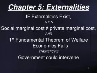
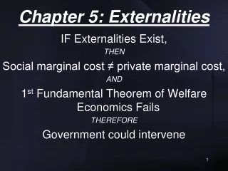
Graphical Analysis, continued • From figure 5.1, as usual, the steel firm maximizes profits at MB=MPC. This quantity is denoted as Q1 in the figure. • Social welfare is maximized at MB=MSC, which is denoted as Q* in the figure.
Graphical Analysis, Implications • Result 1: Q1>Q* • Steel firm privately produces “too much” steel, because it does not account for the damages to the fishery. • Result 2: Fishery’s preferred amount is 0. • Fishery’s damages are minimized at MD=0. • Result 3: Q* is not the preferred quantity for either party, but is the best compromise between fishery and steel firm. • Result 4: Socially efficient level entails some pollution. • Zero pollution is not socially desirable.
Graphical Analysis, Intuition • In Figure 5.2, loss to steel firm of moving to Q* is shaded triangle dcg. • This is the area between the MB and MPC curve going from Q1 to Q*. • Fishery gains by an amount abfe. • This is the area under the MD curve going from Q1 to Q*. By construction, this equals area cdhg. • Difference between fishery’s gain and steel firm’s loss is the efficiency loss from producing Q1 instead of Q*.
Numerical Example: Negative Externalities • Assume the steel firm faces the following MB and MPC curves: • Assume the fishery faces the following MD curve:
Numerical Example, continued • The steel firm therefore chooses Q1: • The socially efficient amount is instead Q*:
Numerical Example, continued • The deadweight loss of steel firm choosing Q1=140 is calculated as the triangle between the MB and MSC curves from Q1 to Q*. • In Figure 5.2, this corresponds to area dhg.
Numerical Example, continued • By moving to Q* the fishery reduces its damages by an amount equal to the trapezoid under the MD curve from Q1 to Q*. • By moving to Q* the steel firm loses profits equal to the triangle between the MB and MPC curve from Q1 to Q*.
Calculating gains & losses raises practical questions • What activities produce pollutants? • With acid rain it is not known how much is associated with factory production versus natural activities like plant decay. • Which pollutants do harm? • Pinpointing a pollutant’s effect is difficult. Some studies show very limited damage from acid rain. • What is the value of the damage done? • Difficult to value because pollution not bought/sold in market. Housing values may capitalize in pollution’s effect.
Private responses • Coase theorem • Mergers • Social conventions
Coase Theorem • Insight: root of the inefficiencies from externalities is the absence of property rights. • The Coase Theorem states that once property rights are established and transaction costs are small, then one of the parties will bribe the other to attain the socially efficient quantity. • The socially efficient quantity is attained regardless of whom the property rights were initially assigned.
Illustration of the Coase Theorem • Recall the steel firm / fishery example. If the steel firm was assigned property rights, it would initially produce Q1, which maximizes its profits. • If the fishery was assigned property rights, it would initially mandate zero production, which minimizes its damages.
Coase Theorem – assign property rights to steel firm • Consider the effects of the steel firm reducing production in the direction of the socially efficient level, Q*. This entails a cost to the steel firm and a benefit to the fishery: • The steel firm (and its customers) would lose surplus between the MB and MPC curves between Q1and Q1-1, while the fishery’s damages are reduced by the area under the MD curve between Q1and Q1-1. • Note that the marginal loss in profits is extremely small, because the steel firm was profit maximizing, while the reduction in damages to the fishery is substantial. • A bribe from the fishery to the steel firm could therefore make all parties better off.
Coase Theorem – assign property rights to steel firm • When would the process of bribes (and pollution reduction) stop? • When the parties no longer find it beneficial to bribe. • The fishery will not offer a bribe larger than it’s MD for a given quantity, and the steel firm will not accept a bribe smaller than its loss in profits (MB-MPC) for a given quantity. • Thus, the quantity where MD=(MB-MPC) will be where the parties stop bribing and reducing output. • Rearranging, MC+MPC=MB, or MSC=MB, which is equal at Q*, the socially efficient level.
Coase Theorem – assign property rights to fishery • Similar reasoning follows when the fishery has property rights, and initially allows zero production. • The fishery’s damages are increased by the area under the MD curve by moving from 0 to 1. On the other hand, the steel firm’s surplus is increased. • The increase in damages to the fishery is initially very small, while the gain in surplus to the steel firm is large. • A bribe from the steel firm to the fishery could therefore make all parties better off.
Coase Theorem – assign property rights to fishery • When would the process of bribes now stop? • Again, when the parties no longer find it beneficial to bribe. • The fishery will not accept a bribe smaller than it’s MD for a given quantity, and the steel firm will not offer a bribe larger than its gain in profits (MB-MPC) for a given quantity. • Again, the quantity where MD=(MB-MPC) will be where the parties stop bribing and reducing output. This still occurs at Q*.
Low transaction costs Few parties involved Source of externality well defined Example: Several firms with pollution Not relevant with high transaction costs or ill-defined externality Example: Air pollution When is the Coase Theorem relevant or not?
Private responses, continued • Mergers • Social conventions
Mergers • Mergers between firms “internalize” the externality. • A firm that consisted of both the steel firm & fishery would only care about maximizing the joint profits of the two firms, not either’s profits individually. • Thus, it would take into account the effects of increased steel production on the fishery.
Social Conventions • Certain social conventions can be viewed as attempts to force people to account for the externalities they generate. • Examples include conventions about not littering, not talking in a movie theatre, etc.
Public responses • Taxes • Subsidies • Creating a market • Regulation
Taxes • Again, return to the steel firm / fishery example. • Steel firm produces inefficiently because the prices for inputs incorrectly signal social costs. Input prices are too low. Natural solution is to levy a tax on a polluter. • A Pigouvian tax is a tax levied on each unit of a polluter’s output in an amount just equal to the marginal damage it inflicts at the efficient level of output.
Taxes • This tax clearly raises the cost to the steel firm and will result in a reduction of output. • Will it achieve a reduction to Q*? • With the tax, t, the steel firm chooses quantity such that MB=MPC+t. • When the tax is set to equal the MD evaluated at Q*, the expression becomes MB=MPC+MD(Q*). • Graphically it is clear that MB(Q*)-MPC(Q*)=MD(Q*), thus the firm produces the efficient level.
Numerical Example: Pigouvian taxes • Returning to the numerical example: • Recall that Q1=140 and Q*=60.
Numerical Example: Pigouvian taxes • Setting t=MD(60) gives t=160. The firm now sets MB=MPC+t, which then yields Q*.
Public responses • Subsidies • Creating a market • Regulation
Subsidies • Another solutions is paying the polluter to not pollute. • Assume this subsidy was again equal to the marginal damage at the socially efficient level. • Steel firm would cut back production until the loss in profit was equal to the subsidy; this again occurs at Q*. • Subsidy could induce new firms to enter the market, however.
Public responses • Creating a market • Regulation
Creating a market • Sell producers permits to pollute. Creates market that would not have emerged. • Process: • Government sells permits to pollute in the quantity Z*. • Firms bid for the right to own these permits, fee charged clears the market. • In effect, supply of permits is inelastic.
Creating a market, continued • Process would also work if the government initially assigned permits to firms, and then allowed firms to sell permits. • Distributional consequences are different – firms that are assigned permits initially now benefit. • One advantage over Pigouvian taxes: permit scheme reduces uncertainty over ultimate level of pollution when costs of MB, MPC, and MD are unknown.
Public responses • Regulation
Regulation • Each polluter must reduce pollution by a certain amount or face legal sanctions. • Inefficient when there are multiple firms with different costs to pollution reduction. Efficiency does not require equal reductions in pollution emissions; rather it depends on the shapes of the MB and MPC curves.
The U.S. response • 1970’s: Regulation • Congress set national air quality standards that were to be met independent of the costs of doing so. • 1990’s: Market oriented approaches have somewhat more influence, but not dominant • 1990 Clean Air Act created a market to control emissions of sulfur dioxide with permits.
Graphical Analysis: Positive Externalities • For simplicity, assume that a university conducts research that has spillovers to a private firm. • Competitive markets, firms maximize profits • Note that university only care’s about its own profits, not the private firm’s. • Private firm only cares about its profits, not the university’s.
Graphical Analysis, continued • MPB = marginal private benefit to university • MC = marginal cost to university • MEB = marginal external benefit to private firm • MSB = MPB+MEB = marginal social benefit
Graphical Analysis, continued • From figure 5.8, as usual, the university maximizes profits at MPB=MC. This quantity is denoted as R1 in the figure. • Social welfare is maximized at MSB=MC, which is denoted as R* in the figure.
Graphical Analysis, Implications • Result 1: R1<R* • University privately produces “too little” research, because it does not account for the benefits to the private firm. • Result 2: Private firm’s preferred amount is where the MEB curve intersects the x-axis. • Firm’s benefits are maximized at MEB=0. • Result 3: R* is not the preferred quantity for either party, but is the best compromise between university and private firm.
Graphical Analysis, Intuition • In Figure 5.8, loss to university of moving to R* is the triangle area between the MC and MPB curve going from R1 to R*. • Private firm gains by the area under the MEB curve going from R1 to R*. • Difference between private firm’s gain and university’s loss is the efficiency loss from producing R1 instead of R*.