Production Planning and Control

Production Planning and Control Chapter 9 Advancement in Production Planning and Control Professor JIANG Zhibin Department of Industrial Engineering & Management Shanghai Jiao Tong University

Chapter 9 Advancement in PPC • Contents • Optimized Production Planning • Theory of Constraint Based Production Planning • Advanced Planning and Scheduling • Mass Customization and its Production Planning

Optimized Production Planning-Introduction (1) • The most prevalent approach in the production planning is based on the concept of material requirement planning (MRP). • The release time is obtained by shifting the expected output time back along the time scale by a period of the estimated average lead time; • The release quantity is derived by dividing the expected output by the estimated average product yield. • However, MRP-based methods have three major drawbacks: • The lead time not only needs to be pre-specified but also is assumed to be static over the entire planning horizon; • The capacity is assumed to be infinite, which means the derived production planning may not be realized; • The production system is made nervous. Little adjustment in MPS changes the due date, requiring the recalculation of MRP.

Optimized Production Planning -Introduction (2) • New methods need to be developed for production planning based on mathematical programming • Time Dimension • Space Dimension: • Corporate level planning: production planning • Shop floor level planning: production lot planning • Mathematical programming based optimized Production Planning Commonly used in production planning: • Linear Programming (LP)- the most widely used methods; • Dynamic Programming (DP)- for multi-periods planning; • Stochastic Programming (SP)-coping with the uncertainty.

Optimized Production Planning -L P (3) Common LP model: x: Decision variables; f(x): Objective function; gi(x): constraints. Commonly used terms: • Objective function, constraints, right-hand side, feasible region, feasible solution, optimal solution. • Features of LP • Linearity: the objective and all constraints can be expressed as a linear function of the decisions variables; • Continuity: the decision variables should be continuous

Profit: $16/kg Profit: $24/kg 3 kg A1 1 barrel of milk 12 hours 4 kg A2 8 hours Optimized Production Planning -L P (4) Example: Make the production planning of milk product One barrel of milk can be made into 3kg A1 by 12 hours or 4kg A2 by 8 hours. The profit of A1 and A2 are $24/kg and $16/kg, respectively. The supply of raw material, milk, is 50 barrels per day. Capacity is 480 hours per day and the production limit of A1 is 100kg at most. 50 barrels of milk/ day, 480 hours available/day, and 100kg A1 at most

x2: barrels of milk to produce A2 x1: barrels of milk to produce A1 Decision variables Objective function Total profit/day: Optimized Production Planning -L P (5) Raw material: Work hours: Constraints Requirement constraints

Xiis continuous: The barrels of milk is real number Optimized Production Planning -L P (6) Model Analysis: • Features of LP: Linearity and Continuity: Proportion: The contributions of xito objective function andconstraints are separately proportional to xi. Addition:The contributions of xi to objective function and constraints are separately independent of xj. The profit/ kg of A1,A2 is constant, and the production quantity and time of A1,A2 from one barrel of milk are constant. The profit/ kg of A1,A2 is constant, and the production quantity and time of A1,A2 from one barrel of milk are constant.

The following are the assumption underlying this model The activity of the model are the production activity on each of wafer fab routes. Activity are measured in terms of the quantity of wafer released; the quantity of output is measured in terms of good die. Each wafer type are assumed to provide a single type of die, thus wafer types and die types are synonymous. There can be alternative wafer fab routes for producing the same wafer type. Optimized Production Planning – An Example in Semiconductor Manufacturing

The following are the assumption underlying this model (Cont.) The overall planning horizon is divided into planning periods in which demands, capacities and productions rates are assumed to be held constant. The length of each planning period for each wafer fab facility may vary and is measured in terms of working days. The length of each period is measured in calendar days for the purpose of discounting cash flows in the objective functions. A production variable is defined as a quantity of a particular wafer type to be released following a particular route during a planning. An inventory variable is defined as the inventory level of a particular die type at the end of a planning period. A backorder variable represents the quantity of die demand that can not be satisfied on time at the end of a planning period. Optimized Production Planning – An Example in Semiconductor Manufacturing

The following are the assumption underlying this model (Cont.) The demands are expressed in terms of time-phased die output requirements and are assumed to be net of initial die inventory and net of equivalent die output of the initial work-in-process (WIP). These demands are divided into prioritized classes that are loaded onto front end facilities by incremental LP calculation. Demands in class 1 are loaded first, then demands in classes 1 and 2 loaded subject to not exceeding backorder levels associated with class 1, etc. The formulation for all classes is the same, except for the values of the demands and the lower bounds on back order variables. Production is rate-based, i.e., the release quantity in a particular period is to be distributed uniformly over the period. Optimized Production Planning – An Example in Semiconductor Manufacturing

The following are the assumption underlying this model (Cont.) As a horizon condition, the wafer fab are required to enter steady-state, whereby production releases on each route are required to follow some constant rate in all periods falling within one total flow time of the planning horizon. The planning periods that overlap the interval beginning one total flow time for a route before the planning horizon until the horizon are termed frozen periods with respect to that route. Demands from each class in the last planning period are assumed to continue at the same rate forever. Optimized Production Planning – An Example in Semiconductor Manufacturing

Optimized Production Planning – An Example in Semiconductor Manufacturing • Parameters • g: die type. • i: wafer fab route. • l: processing step (i. e., operation) on a wafer fab route. • li: the last step on wafer fab route i. • k: resource type (i. e., machine type). • p, q: planning period, p = 1,2,…，P. P is the planning horizon. An extra period P+1 is appended to the planning horizon whose length is equal to the flow time of the longest fab route. • r: demand class, r = 1，2，…，R. • Gr: set of all die types appearing in r-th demand class. • I r: set of all wafer routes producing die types appearing in Gr. • Kr: set of all resource types loaded by routes in I r.

Optimized Production Planning – An Example in Semiconductor Manufacturing The following values are assumed to be known and constant

Optimized Production Planning – An Example in Semiconductor Manufacturing Continued

Optimized Production Planning – An Example in Semiconductor Manufacturing Variables: Short notation:

Optimized Production Planning – An Example in Semiconductor Manufacturing Maximize the discounted sum of (die output revenue)-(raw material cost)-(die inventory holding cost)-(cost of backordered die demands) Objective function (For r-th demand class) Constraints: • Conservation of Die Demand； • Constraints relating Resource Capacity； • Variables ranges.

Optimized Production Planning – An Example in Semiconductor Manufacturing (die output during the period) – (inventory at the end of period) + (backorders at the end of period) = (demands at the end of period) (die output during the period) + (inventory at the start of period) – (backorders at the end of period) – (inventory at the end of period) + (backorders at the end of period) = (demands at the end of period) (die output during the period) – (backorders at the end of period) + (backorders at the end of period) = (demands at the end of period) Constraints: Conservation of Die Demand； Constraints relating Resource Capacity； Variables ranges.

(machine hours required to process new releases)≤ (available machine hours for processing activity) – (machine hours required to flush initial WIP) Optimized Production Planning – An Example in Semiconductor Manufacturing Constraints: Conservation of Die Demand； Constraints relating Resource Capacity； Variables ranges. 0 ≤(backorder variables)≤ ( upper bound on backorder quantity), and all other variables≥0.

DP is an approach developed to solve sequential, or multi-stage, decision problems by solving a series of single stage problems; DP tends to break the original problem to sub-problems and chooses the best solution in the sub-problems, beginning from the smaller in size; DP follows “ the principle of best”, that is the best solution of the problem will come by the combination of the best solutions of sub-problems, if the possible solutions of a problem are a combination of possible solutions of sub-problems DP can solve the multi-periods production planning problems. Optimized Production Planning -Dynamic Programming (DP)

SP is a framework for modeling optimization problems that involve uncertainty; The most widely applied and studied stochastic programming models are two-stage linear programs; Multi-stage linear programs have been extended, SP can tackle the uncertainty of future demand. Optimized Production Planning -Dynamic Programming (DP) The decision makers take some actions at the first stage; A recourse decision can then be made in the second stage that compensates for any bad effects that might have been experienced as a result of the first-stage decision. Each stage consists of a decision followed by a set of observations of the uncertain parameters which are gradually revealed over time.

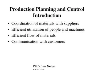
APS-Overview of Planning and Scheduling • Generally speaking, planning and scheduling jointly determine how, when, and in what quantity products will be manufactured or purchased. In essence, planning establishes what should be done and scheduling determines how to do it; • There is no agreed definition of planning versus scheduling. Many believe that the right and only way to achieve accurate due dates is to perform very detailed scheduling. Others believe that it is much more important to put more effort in the planning process. But most agree that the distinction between planning and scheduling is the trade-off of time horizon versus the level of detail.

APS- Definition Advanced Planning and Scheduling (APS) is a software system that uses intelligent analytical tools to perform finite scheduling and produce realistic plans.

APS-Overview (1) • Its most important advantage over traditional planning approaches is that material and capacity are simultaneously considered as elements that may constrain production. This stands in marked contrast to the conventional MRP approach of independently planning material and then subsequently checking this plan against capacity to identify violations; • APS systems are able to generate plans and schedules very quickly. An APS engine can be designed to either look over a long time horizon (a few months) with less details or more details over a shorter period (a few weeks). • APS covers various capabilities such as “finite capacity scheduling” or “constraint-based scheduling” at shop floor level; • Quite intuitive to say that the APS systems resolve (or attempt to resolve) the shortfall of the ERP system as a planning tool;

APS-Overview (2) • APS does Advanced Planning • Consider business objectives • Consider the organization of machines and work cells • APS does Advanced Scheduling • Consider plant capacity • Consider business limitations

APS-the Scope (1) • The scope of APS is not limited to factory planning and scheduling, but has grown rapidly to include the full spectrum of enterprise and inter-enterprise planning and scheduling functions: • Strategic and long-term planning • Demand planning and forecasting • Sales and operations planning (SOP) • Inventory planning • Supply chain planning (SCP) • Available-to-promise (ATP)

APS-the Scope (2) • Manufacturing planning • Distribution planning • Transportation planning • Production scheduling • Shipment scheduling • Inter-company collaboration • —Source: Bermudez, John. “Advance Planning and Scheduling: Is It as Good as It Sounds?” The Report on Supply Chain Management. Advanced Manufacturing Research, Inc., March, 1998.)

Enterprise Wide Planning Available to Supply Promise Chain Planning Capable to Production Promise Scheduling APS- the Four-Part Model AMR’s APS Model — Source: Advanced Manufacturing Research, Inc.

APS- Mathematical Technologies • Linear Programming • Genetic Algorithms • Heuristics • Constraint Based Programming (CBP) • —Source: Shires, Nigel, (2005). “Optimization Techniques and Their Application to Production Scheduling ,” White Paper, Preactor International, published on website: http://www.preactor.com/whitepapers.asp.

APS-APS/ERP Integration • The comprehensive nature of today’s APS algorithms drives the need for copious amounts of data--data that typically reside in an ERP system. This means that attaining the full benefits of APS is largely predicted on how well it is integrated with ERP. When done well, both systems benefit. • —Source: Musselman, K., and Uzsoy, R. (2001), “Advanced Planning and Scheduling for Manufacturing,” in Handbook of Industrial Engineering, 3rd Ed., G. Salvendy, Eds., John Wiley & Sons, New York.

APS/ERP Integration APS/ERP Integration • —Source: Musselman, K., and Uzsoy, R. (2001), “Advanced Planning and Scheduling for Manufacturing,” in Handbook of Industrial Engineering, 3rd Ed., G. Salvendy, Eds., John Wiley & Sons, New York.

APS- Software Providers • Preactor • SAP - Advanced Planner and Optimizer (APO) • Oracle - APS • Manugistics • i2 • …

APS-Preactor APS Screenshot

APS-SAP-APO Screenshot

The theory was first described by Israel’s physicist Dr. Eliyahu M. Goldratt in his book The Goal as a way of managing the business to increase profits in 1980’s. Theory of Constraints (TOC)-Introduction TOC is a proven method that can be used by existing personnel to increase throughput (sales), reliability, and quality while decreasing inventory, WIP, late deliveries, and overtime. Successful organizations also adopt TOC to help make tactical & strategic decisions for continuous improvement.

The Theory of Constraints is based on the premise that: “Every real system, such as a business, must have within it at least one constraint. If this were not the case then the system could produce unlimited amounts of whatever it was striving for, profit in the case of a business.……………….” Dr Eli Goldratt TOC-Introduction

TOC-Drum Buffer Rope buffer • Drum Buffer Rope (DBR) is a planning and scheduling solution derived from the Theory of Constraints (TOC). • The fundamental assumption of DBR is that within any plant there is one or a limited number of scarce resources which control the overall output of that plant. This is the “drum”, which sets the pace for all other resources. • In order to maximize the output of the system, planning and execution behaviors are focused on exploiting the drum, protecting it against disruption through the use of “time buffers”, and synchronizing or subordinating all other resources and decisions to the activity of the drum through a mechanism that is akin to a “rope”. rope drum

Step 1: Identify the system's constraint(s) Step 2: Decide how to exploit the system’s constraint(s) Step 3: Subordinate everything else to the above decision Step 4: Elevate the system’s constraint(s) Step 5: If in the previous step, a constraint has been broken go back to step 1, but do not allow inertia to become the system’s constraint TOC-the Steps for Implementation

A constraint is anything in an organization that limits it from moving toward or achieving its goal. There are two basic types of constraints: physical constraints and non-physical constraints. A physical constraint is something like the physical capacity of a machine. A non-physical constraint might be something like demand for a product, a corporate procedure, or an individual's paradigm for looking at the world. THE MARKET CAPACITY RESOURCES SUPPLIERS FINANCE KNOWLEDGE OR COMPETENCE POLICY TOC- Types of Constraint:

1. Production Planning and Scheduling 2. Distribution and Supply Chain 3. Financial Management 4. Marketing 5. Strategic Planning 6. Project Management TOC- Applications

Factory production rate is production rate of bottleneck work center; Most of the buffer WIP should be waiting at bottleneck; Bottleneck implies certain amount of idle time at other work stations; Important to regulate bottleneck workload; other work centers should serve the bottleneck, not optimize themselves. TOC-the Principles of Applying TOC in Production Scheduling

Capacity is defined as the available time for production (excluding maintenance and other downtime) Abottleneck(constraint) is defined as any resource whose capacity is less than the demand placed upon it A non-bottleneckis a resource whose capacity is greater than the demand placed on it A capacity-constrained resource (CCR) is one whose utilization is close to capacity and could be bottleneck if it is not scheduled carefully TOC-Capacity and Bottlenecks in Production

SLIM (Short Cycle Time and Low Inventory in Manufacturing) is a project carried by Prof. Leachman at University of California at Berkeley. SLIM is a set of methodologies and scheduling applications for managing cycle time in semiconductor and its main method is TOC. Between 1996 and 1999, Samsung Electronics Corp., Ltd., implemented SLIM in all its semiconductor manufacturing facilities and achieve great success: During the presentation at the 2001 Franz Edelman Award Competition, Yoon-Woo Lee, president of Samsung’s semiconductor business, stated: “The financial impact of SLIM was significant. We increased revenue almost $1 billion dollars through five years without any additional capital investment, and our global DRAM market share increased from 18 percent to 22 percent.” TOC- An Example in Semiconductor Manufacturing

Photo Layer j+1 Photo Layer j+2 Photo Layer j-1 Photo Layer j Wip level TOC- An Example in Semiconductor Manufacturing WIP between photo steps at normal time Fab Process The pipe represents the production line, and its width represents the maximum flow rate or capacity at various process steps. SEC fabs were designed so that the photo machines are the bottlenecks, and other machines have surplus capacity. Thus the pipe in the figure narrows at each photo step. When all the machines are up and the process is in control, the photo machines are the bottlenecks, and the largest concentrations of WIP is at those points.

Fab Process Process trouble Photo Layer j+1 Photo Layer j+2 Photo Layer j-1 Photo Layer j Wip level Photo Layer j+1running out TOC- An Example in Semiconductor Manufacturing WIP between photo steps at disturbance The case of process or equipment trouble at a non-photo manufacturing area of the fab is depicted by a constriction of the pipe at a non-photo step. If this condition persists, the WIP at a photo machine can become exhausted. A buffer is needed, proportional to the risk of trouble in that layer. For example, if Layer j of the process experiences more trouble than Layer j+1 the bottleneck step immediately following Layer j should be awarded a larger buffer than the bottleneck step following Layer j+1.

The philosophy underlying SLIM is to distribute WIP to put the fab in the best position to cope with the next disruption. That is, while the equipment and process are working well, the fab should strive to move as much WIP as possible to the photo bottleneck, to be prepared for the next disruption. TOC- An Example in Semiconductor Manufacturing The way to solve the problem

With the increasing competition in the global market, the manufacturing industry has been facing the challenge of increasing customer value; More importantly, quality means ensuring customer satisfaction and enhancing customer value to the extent that customers are willing to pay for the goods and services; A well-accepted practice in both academia and industry is the exploration of flexibility in modern manufacturing systems to provide quick response to customers with new products catering to a particular spectrum of customer needs; The key to success in the highly competitive manufacturing enterprise often is the company’s ability to design, produce, and market high-quality products within a short time frame and at a price that customers are willing to pay; In order to meet these pragmatic and highly competitive needs of today’s industries, it is imperative to promote high-value-added products and services; Mass customization enhances profitability through a synergy of increasing customer-perceived values and reducing the costs of production and logistics. CS-Introduction

Mass customization is “producing goods and services to meet individual customer’s needs with near mass production efficiency”; Mass customization is a new paradigm for industries to provide products and services that best serve customer needs while maintaining near-mass production efficiency. Contradicted two sides: CS-Introduction • Mass production demonstrates an advantage in high-volume production; • Satisfying each individual customer’s needs can often be translated into higher value, however, economically not viable;

Mass customization is capable of reducing costs and lead time by accommodating companies to garner economy of scale by repetitions. With flexibility and programmability, companies with low to medium production volume can gain an edge over competitors by implementing MC; Mass customization can potentially develop customer loyalty, propel company growth, and increase market share by widening the product range. CS-Introduction Economic Implication of Mass Customization

The essence of mass customization lies in the product and service providers’ ability to perceive and capture latent market niches and subsequently develop technical capabilities to meet the diverse needs of target customers; To encapsulate the needs of target customer groups means to emulate existing or potential competitors in quality, cost, quick response; Therefore, the requirements of mass customization depend on three aspects: time-to-market (quick responsiveness), variety (customization), and economy of scale (volume production efficiency); Successful mass customization depends on a balance of three elements: features,cost, and schedule. CS-Introduction Technical challenges

Production Planning and Control