Analytical vs. Numerical Minimization
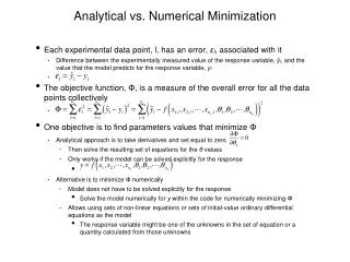
Analytical vs. Numerical Minimization. Each experimental data point, l, has an error, ε l , associated with it Difference between the experimentally measured value of the response variable, ŷ l , and the value that the model predicts for the response variable, y l

Analytical vs. Numerical Minimization
E N D
Presentation Transcript
Analytical vs. Numerical Minimization • Each experimental data point, l, has an error, εl, associated with it • Difference between the experimentally measured value of the response variable, ŷl, and the value that the model predicts for the response variable, yl • The objective function, Φ, is a measure of the overall error for all the data points collectively • One objective is to find parameters values that minimize Φ • Analytical approach is to take derivatives and set equal to zero • Then solve the resulting set of equations for the θ values • Only works if the model can be solved explicitly for the response • Alternative is to minimize Φ numerically • Model does not have to be solved explicitly for the response • Solve the model numerically for y within the code for numerically minimizing Φ • Allows using sets of non-linear equations or sets of initial-value ordinary differential equations as the model • The response variable might be one of the unknowns in the set of equation or a quantity calculated from those unknowns
MATLAB Template Files for Single Response Data • FitNonlinSR.m (fit a non-linear equation to single response data) • Model: • FitNumAlgSR.m (numerically fit a set of non-linear (algebraic) equations to single response data) • Model: • Response:
FitNumDifSR.m (numerically fit a set of initial-value ordinary differential equations to single response data) • Model: • Response: • Output • Best value for each parameter • Correlation coefficient, r2 • 95% confidence interval for each parameter • Plot(s) • Model plot if there is only one set variable • Parity plot and residuals plots if there are more than one set variables • The template files must be modified each time they are applied to a new problem
Required Information and Data • FitNonlinSR.m • a set of experimental data points, each of which consists of a value for the response variable, ŷ, and corresponding values for each of the set variables xi • a guess for the value of each unknown parameter that appears in the model • code that calculates the model-predicted value of the response variable, given values for the parameters and values for the set variables • FitNumAlgSR.m • first two items above • code that evaluates the set of non-linear equations to be solved, given values for the unknowns • code that provides a guess for the values of the unknowns • FitNumDifSR.m • first two items above • code that evaluates the derivatives in the set of initial value ordinary differential equations given values of the independent and dependent variables • code that provides the initial values of the independent and dependent variables • code that provides the final value of the independent variable
A Note on Numerical Minimization • An objective function may have more than one “local” minimum and maximum • The analytical approach (taking the derivatives analytically and solving the resulting equations) will find all minima and maxima of the objective function (red arrows) • The numerical algorithm, as described here, will only find one minimum • It could be the global minimum • It could be a local minimum • It is advisable to repeat a regression analysis using very different guesses for the parameters to see whether the algorithm finds the same minimum or different ones
Fitting Models to Multiple Response Data • The objective function differs depending upon the nature of the data • Here only consider a complete data set where every response variable was measured in every experiment • In this case, • MATLAB template files (requiring complete data set) • Analogous to FitNumAlgSR.m and FitNumDifSR.m • filenames end with MR.m instead of SR.m • Correlation coefficient and 95% confidence intervals for parameters are not computed

